Calculating powder X-ray diffraction in the browser
Double-precision powder diffraction with pymatgen as the reference. Shorter scheduling waits reduce the warmed silicon task median from 78.2 to 3.5 ms, with matching peak tables.
2026-10-01 · Mol2Mat · revision 1
Calculating powder patterns from crystal structures
A crystal's lattice and atomic coordinates can be used to calculate its powder X-ray diffraction peak positions and relative intensities. The lattice determines where peaks appear; atom types, positions and occupancies determine which reflections are enhanced or extinguished. These patterns help compare candidate database structures. Sample, temperature and instrumental conditions also matter when comparing them with experiments.
Mol2Mat implements this calculation in double-precision TypeScript and runs it in a dedicated Web Worker, with XRDCalculator in pymatgen 2026.9.23 as the reference.[1] The two implementations use identical structures and conditions, then compare angles, interplanar spacings, relative intensities and hkl families peak by peak. Thirty-nine test inputs include nonempty patterns, empty intervals and out-of-range inputs. The maximum angular difference is 1.4211×10⁻¹³°.[2]
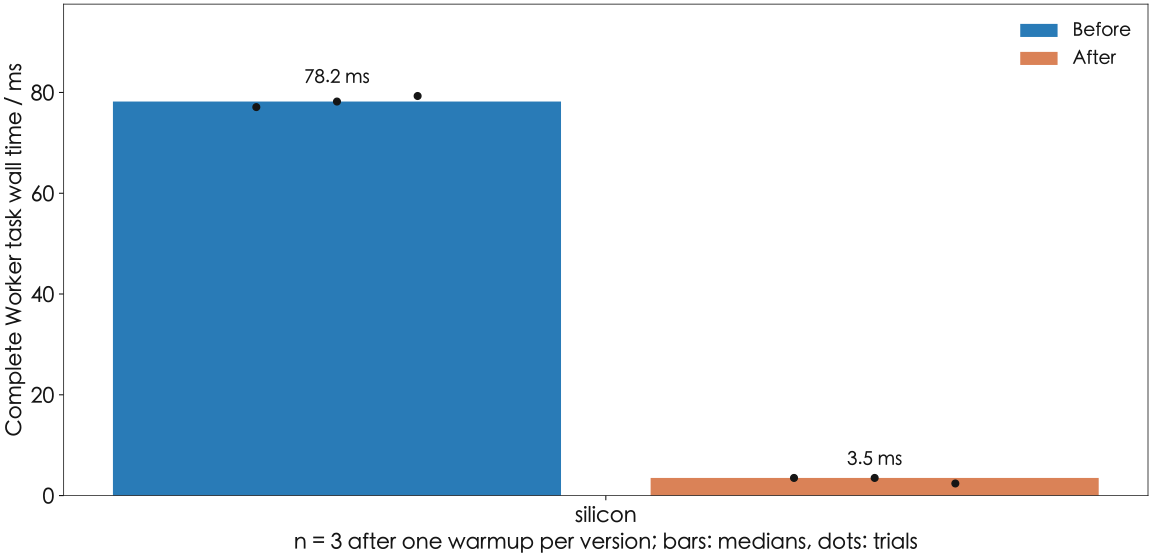
Optimization reduces time in two places: Friedel symmetry and scattering-factor reuse avoid repeated arithmetic, while event-loop scheduling shortens waits between progress notifications. For the warmed silicon test, median Worker task time falls from 78.2 to 3.5 ms. Both versions return identical scientific results and retain all 21 progress notifications.[5]
Lattice, structure factors and powder intensity
Let the columns of lattice matrix A be real-space basis vectors, using a reciprocal-lattice convention with the 2π factor omitted. For integer indices h = (h, k, l), the reciprocal vector, interplanar spacing and Bragg condition are:
Cell lengths and wavelength are in Å; degrees and radians are converted at display and trigonometric boundaries.
Atomic scattering factors use pinned element-specific coefficients. With s = sinθ/λ, occupancy o_j and fractional position r_j:
Species sharing a site contribute coherently through their own scattering factors and occupancies; vacancies contribute zero scattering.
After accumulating reflections at the same angle, the calculation uses the reference Lorentz–polarization factor:
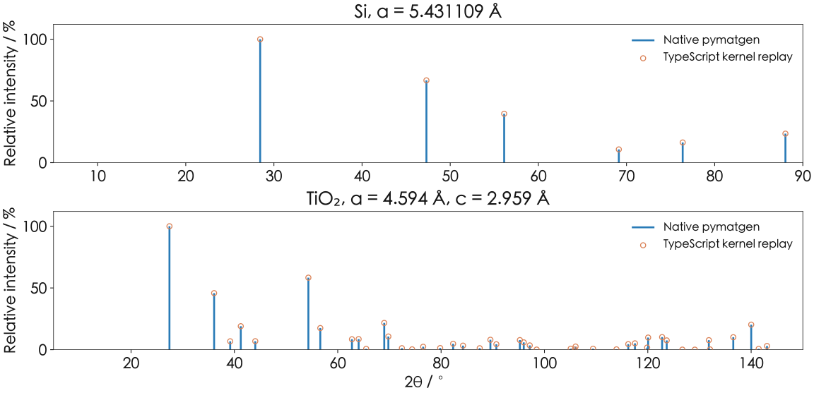
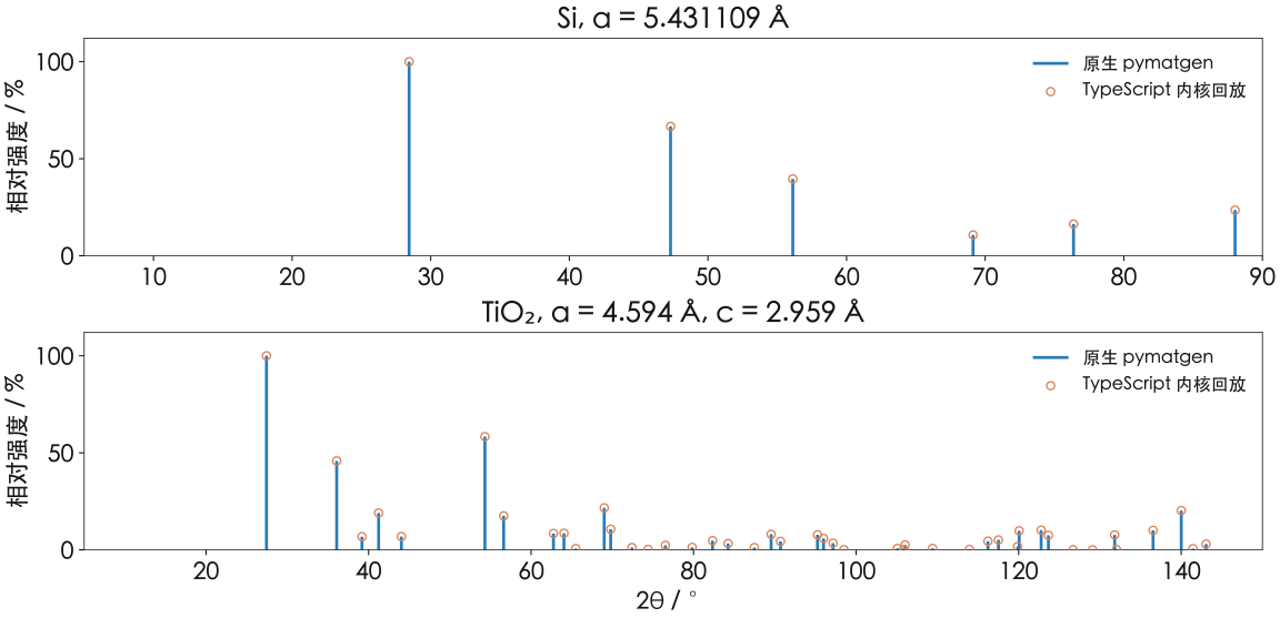
The largest peak across the reference range is normalized to 100. The figure displays calculated discrete reflections of synthetic cells, with heights in relative-intensity units.
Reflection enumeration and double-precision calculation
The kernel implements the reference numerical sequence directly and loads scattering coefficients as a hashed asset. JavaScript Number supplies IEEE 754 double precision for peak positions and structure-factor accumulation. The Worker handles calculation and cooperative cancellation.
Wavelength and maximum angle limit the reciprocal-vector lengths that need to be checked. The calculation first builds conservative integer bounds from real-space basis lengths, then filters by actual reciprocal length. This also handles non-orthogonal cells. Under the current normal-scattering approximation, Friedel partners have equal intensity, so half the indices can be enumerated and their paired contributions restored. At each reflection, atoms of the same element can share a single scattering-factor calculation.
Peak merging uses 10⁻⁵° angular bins and explicitly reproduces NumPy’s ties-to-even rounding. The relative-intensity cutoff remains 0.001%. A whole-pattern maximum unnormalized intensity in (0, 10⁻⁸) returns a numerical-resolution limitation. Enumeration and normalization cover 0–150° before cropping to the requested subrange within 5–150°; cropped peaks retain the full-pattern intensity scale.
Input handling preserves the supplied lattice, atoms and occupancies, with symprec = 0 by default. Missing lattices, singular cells, unknown scattering elements, excessive occupancies and assembled structures return their respective limitation reasons. Hexagonal cells retain four-index notation and family multiplicities; acceptance checks both peak tables and family sets.
Reference inputs and peak-table comparisons
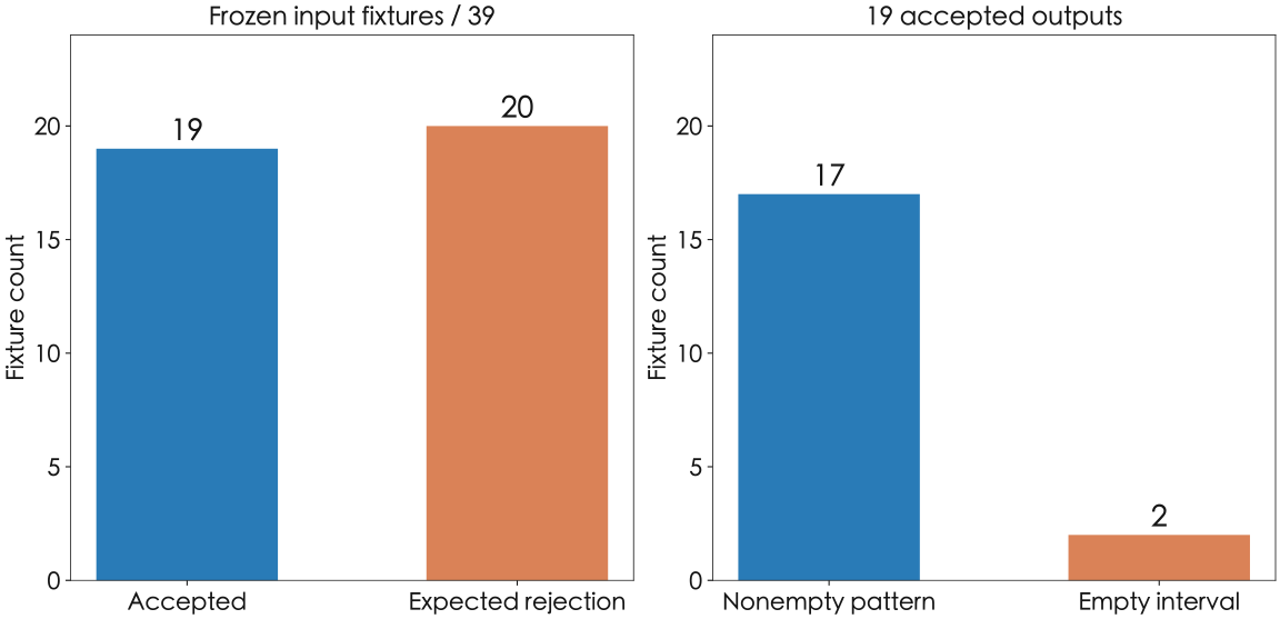
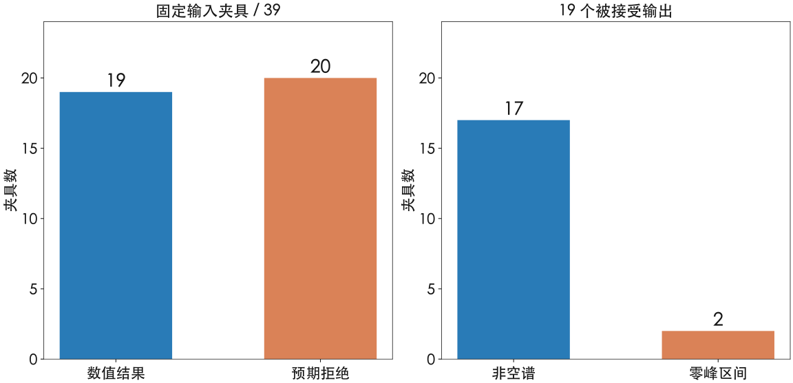
The native reference pins pymatgen and scattering-coefficient versions. Thirty-nine fixtures comprise 19 accepted results and 20 expected rejections, with two empty peak intervals among the accepted cases. Constructed cells cover silicon, gold, rutile, hexagonal titanium, a triclinic cell, mixed occupancies, allowed duplicate sites, vacancies, multiple wavelengths and the 200-site boundary.[2]
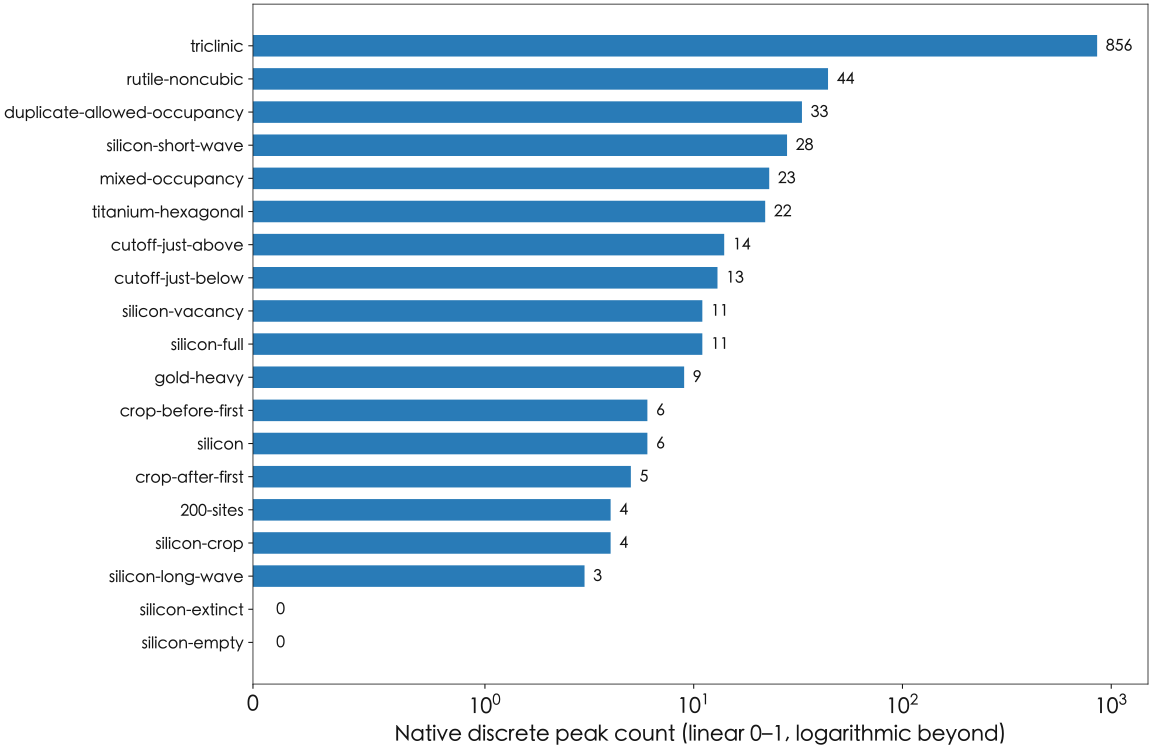
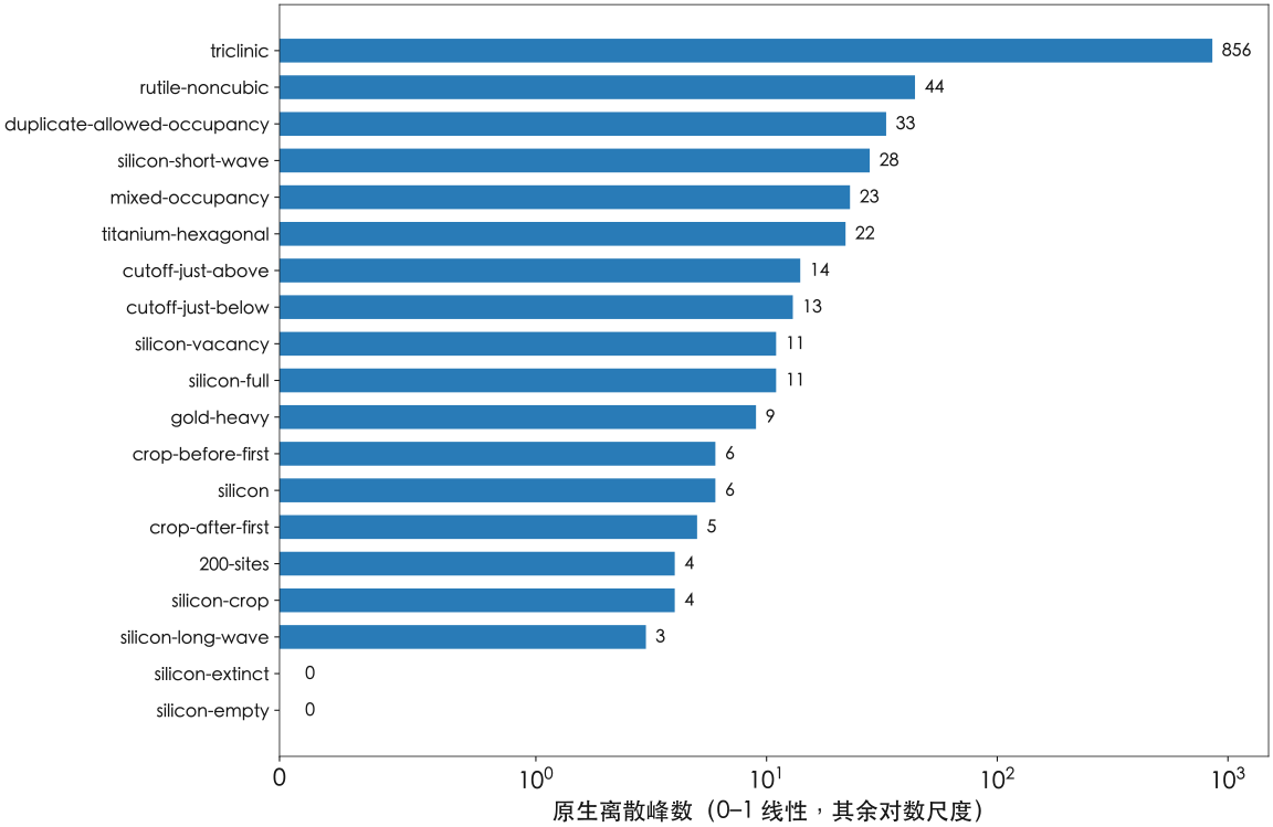
The triclinic fixture contains 856 discrete peaks, exercising general reciprocal geometry and family grouping. Inputs around intensity thresholds and the first-peak crop boundary test peak-membership sensitivity to small numerical changes. All 20 rejection reasons are compared individually, extending the checks to input acceptance rules.
Each fixture preserves its input, native output, reference timing and SHA-256. TypeScript replay checks peak tables, family sets and input immutability for all 39 inputs. Actual distribution Workers provide separate protocol and timing checks.
Differences in peak positions, spacings and intensities
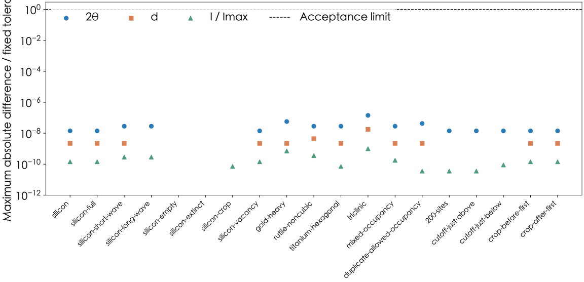
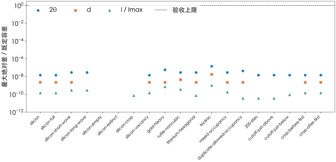
Acceptance compares individual peaks. Peak counts, membership and hkl family sets must agree; 2θ, d and relative intensity use the pre-existing absolute tolerances below. The intensity tolerance applies to the 0–100 numerical scale.
Across the 19 accepted inputs, maximum differences in angle, spacing and intensity are 1.4211×10⁻¹³°, 1.7764×10⁻¹⁵ Å and 9.9476×10⁻¹⁴. All 39 tests pass, including expected rejections. The plotted differences show that the two double-precision programs give closely matching results for the same structure. The accuracy of the structural parameters depends on their source and measurement conditions.
Actual product exports also cover six peaks for COD 1512541 and fourteen for JARVIS dft_3d_JVASP-1002. Both have a maximum angular difference of 2.8422×10⁻¹⁴° against native pymatgen. These records use theoretical structures and preserve their individual cell parameters, provenance and hashes.[2,3,4]
| Field | Absolute tolerance | Maximum absolute difference |
|---|---|---|
| 2θ / ° | 1×10⁻⁶ | 1.4211e-13 |
| d / Å | 1×10⁻⁷ | 1.7764e-15 |
| Relative intensity / 0–100 | 1×10⁻⁴ | 9.9476e-14 |
| Peak membership, hkl families | Exact | All equal |
Progress notifications and event-loop scheduling
A Worker task has to send progress, handle messages and return results as well as perform the calculation. Total time can be divided into:
When the calculation itself is short, waiting repeatedly to yield the event loop can take most of the time.
The old task host awaited setTimeout(0) after each progress notification to give the event loop a chance to process cancellation. Repeated nested timers encounter a minimum delay, so these short waits accumulate with every notification. An isolation test kept the kernel and progress count fixed while changing only the yield mechanism, confirming the scheduling overhead.[5]
The new host schedules yields through a task-local MessageChannel, giving message handling a chance to run while avoiding repeated timer waits. It checks cancellation before and after each yield and preserves progress sequence, stages and result-commit order. On completion, it closes the ports and settles progress notifications. The host still controls termination of synchronous external kernels.
Paired timings for the silicon task
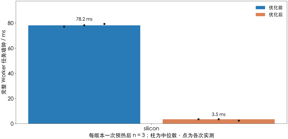
Old and new distribution Workers alternate the silicon fixture in the same macOS Chromium session, with one warmup and three measured trials per version. Old observations are 77.1, 78.2 and 79.3 ms; new observations are 3.5, 3.5 and 2.4 ms. The median falls from 78.2 to 3.5 ms, a 95.5% reduction and approximately 74.7 ms saved.[5]
Both versions retain all 21 progress events and identical scientific fields; device-self-test time is the sole field removed from comparison. Seventeen current distribution checks cover Worker protocol, storage, domain and numerics. Cancellation takes approximately 1.1 ms and retry succeeds. All 39 frozen fixtures retain their original position, spacing and intensity tolerances.
These measurements use a warmed Worker. The silicon calculation is short, so waits between progress notifications have a large effect on total time. A larger enumeration range spends more time calculating structure factors, changing the proportion saved by scheduling. The figure includes all three observations on the shared development machine so that run-to-run variation remains visible.
| Input | Before / ms | After / ms | Time reduction |
|---|---|---|---|
| silicon | 78.2 | 3.5 | 95.5% |
Calculation costs for different cells
Enumeration cost depends jointly on reciprocal-space candidates and site count. The current domain is an explicit three-dimensionally periodic cell with 1–200 sites, wavelength 0.5–3 Å and angle intervals within 5–150°. The integer box permits up to 250000 candidates and candidates times sites up to 5000000. Large cells can produce dense reciprocal points even with few atoms.
Historical single observations give approximately 1.89 ms for the silicon Node kernel and 9.11 ms for native Python; the 200-site fixture takes approximately 27.89 and 35.31 ms. The table preserves these n = 1 cost records, with each native and Node timing entry point available in the data.
Product receipts record task times of 0.135 s for COD and 0.081 s for JARVIS. Independent Python verification also includes work such as initialization, so these records measure different processes. The preceding section's paired measurements, from task submission to result transfer, establish the optimization's effect. Historical records describe the cost of different inputs.
| Fixture | Node / ms | Python / ms |
|---|---|---|
| silicon | 1.894 | 9.111 |
| rutile-noncubic | 0.548 | 3.795 |
| triclinic | 4.806 | 8.720 |
| 200-sites | 27.886 | 35.311 |
Scope of the structural calculation
The calculation uses the kinematic approximation and produces discrete powder reflections determined by the lattice, atomic scattering factors, occupancies and Lorentz–polarization correction. Anomalous scattering, thermal displacement, crystallite size, microstrain, preferred orientation, diffuse and multiple scattering, and instrument response are subjects for additional modelling.
Structural provenance can affect patterns much more than porting error. Relaxed theoretical cells, cells measured at different temperatures and defective samples may share a formula yet yield different positions and intensities. Comparisons should fix the lattice, atomic coordinates, occupancies, wavelength and normalization range while preserving structural identity.
The implementation serves structure previews, discrete-peak comparisons and reference-calculation reproduction. Experimental fitting, Rietveld refinement and quantitative phase analysis additionally require peak-shape, background, instrument and sample models, together with independent experimental patterns.
Data, provenance and reproducible checks
Downloads contain 39 native fixtures, TypeScript kernel replay, peak CSVs, product comparisons and source hashes. Lossless JSON preserves raw output; CSVs retain values before display rounding. Figures and acceptance checks use the same peak tables.
Run node scripts/technical-notes/replay_xrd.mjs from the repository root to recompute the current kernel. After extracting the independent bundle, python replay.py --article xrd compares saved peaks, hkl families and the three numerical fields.
optimization.json and optimization.csv provide every old/new Worker observation, distribution identities and scientific-output checks. python optimization-replay.py verifies file hashes, warmup exclusion, medians, progress events and result equality.[5]
浏览器端粉末 X 射线衍射计算与参考实现对照
以 pymatgen 为参考实现双精度粉末衍射计算。减少调度等待后,预热硅任务的中位耗时从 78.2 ms 降至 3.5 ms,峰表保持一致。
2026-10-01 · Mol2Mat · revision 1
从晶体结构计算粉末衍射谱
从晶格和原子坐标出发,可以计算晶体的粉末 X 射线衍射峰位与相对强度。晶格决定峰出现在什么角度,原子种类、位置与占位决定哪些反射增强或消失。这样的计算谱便于比较数据库中的候选结构;与实验谱比较时,样品、温度和仪器条件也会影响结果。
Mol2Mat 用双精度 TypeScript 实现这套计算,在专用 Web Worker 中运行,并以 pymatgen 2026.9.23 的 XRDCalculator 作对照。[1] 对同一结构和计算条件,两套程序逐峰比较角度、晶面间距、相对强度和 hkl 家族。39 个测试输入包括正常谱、没有衍射峰的区间和超出范围的输入,最大峰位差为 1.4211×10⁻¹³°。[2]
优化从两处减少耗时:利用 Friedel 对称性和散射因子复用减少重复运算,调整事件循环调度以缩短进度通知之间的等待。在预热后的硅测试中,Worker 任务中位耗时从 78.2 ms 降至 3.5 ms。两版返回相同的科学结果,也保留了全部 21 次进度通知。[5]
晶格、结构因子与粉末强度
令晶格矩阵 A 的列为实空间基矢,采用省略 2π 因子的倒易晶格约定。对整数指标 h = (h, k, l),倒易矢量、晶面间距与 Bragg 条件为:
晶胞长度和波长以 Å 表示,度与弧度在显示和三角函数边界转换。
原子散射因子使用固定的元素系数。令 s = sinθ/λ,位点占位为 o_j,分数坐标为 r_j,则:
同位点的不同元素按各自散射因子与占位作相干求和,空位的散射贡献为零。
同一角度的反射累积后,采用参考程序的 Lorentz–polarization 因子:
全参考范围的最大峰归一化为 100。下图展示合成晶胞的计算离散峰,峰高的单位为相对强度。
反射枚举与双精度计算
内核直接实现参考数值步骤,散射系数以带哈希的数据资产加载。JavaScript Number 提供 IEEE 754 双精度,峰位计算与结构因子累积沿用这一精度;Worker 负责计算和协作取消。
波长与最大衍射角限定了需要检查的倒易矢量长度。程序先由实空间基矢长度构造足够大的整数枚举范围,再按实际倒易长度筛选,因此也能处理非正交晶胞。在当前正常散射近似下,Friedel 对具有相同强度:只需枚举一半指标,再计入成对贡献。同一反射中,同元素的散射因子也可以共用一次计算。
峰合并使用 10⁻⁵° 角度分箱,并显式实现 NumPy 的 ties-to-even 中点舍入。相对强度截断沿用 0.001%。全谱最大未归一化强度处于 (0, 10⁻⁸) 时,浏览器返回数值分辨率限制。内核先在 0–150° 范围枚举和归一化,再裁剪到请求的 5–150° 内子区间;裁剪谱沿用全谱强度标尺。
输入处理保持原始晶格、原子与占位,默认 symprec = 0。缺失晶格、奇异晶胞、未知散射元素、超额占位和组合结构分别返回限制原因。六方晶胞保留四指标表示与家族重数,验收同时检查峰表和家族集合。
参考输入与峰表对照
原生对照固定 pymatgen 与散射系数版本。39 个夹具包含 19 个可接受结果和 20 个预期拒绝输入;可接受结果中有两个零峰区间。构造晶胞覆盖硅、金、金红石、六方钛、三斜晶胞、混合占位、允许的重复位点、空位、不同波长和 200 位点边界。[2]
三斜夹具含 856 个离散峰,用于检查一般倒易晶格和峰家族归并。强度阈值上下与第一峰裁剪边界分别检查峰成员对微小数值变化的敏感性。20 个拒绝输入逐项比较原因,使数值检查同时覆盖输入接受规则。
每个夹具保存原始输入、原生结果、参考耗时与 SHA-256。TypeScript 回放逐项检查 39 个输入的峰表、家族集合及输入不变性;浏览器 Worker 的协议与计时另由实际分发包验证。
峰位、间距和强度的数值差
验收逐峰比较。峰个数、成员关系和 hkl 家族集合要求相同;2θ、d 与相对强度使用下表中的既定绝对容差。强度容差作用于 0–100 的数值标尺。
19 个可接受输入中,峰位、间距和强度的最大差分别为 1.4211×10⁻¹³°、1.7764×10⁻¹⁵ Å 和 9.9476×10⁻¹⁴。39 个测试全部通过,包括预期拒绝的输入。图中的差值说明两套双精度程序对同一结构给出接近的结果;结构参数是否准确,则取决于结构来源和测量条件。
真实产品导出还覆盖 COD 1512541 的 6 个峰与 JARVIS dft_3d_JVASP-1002 的 14 个峰;相对原生 pymatgen,两者最大角度差均为 2.8422×10⁻¹⁴°。这两条记录使用理论结构,各自保存晶格参数、来源与哈希。[2,3,4]
| 字段 | 绝对容差 | 最大绝对差 |
|---|---|---|
| 2θ / ° | 1×10⁻⁶ | 1.4211e-13 |
| d / Å | 1×10⁻⁷ | 1.7764e-15 |
| 相对强度 / 0–100 | 1×10⁻⁴ | 9.9476e-14 |
| 峰成员、hkl 家族 | 精确一致 | 全部一致 |
进度通知与事件循环调度
一次 Worker 任务除了计算,还要发送进度、处理消息和交回结果。总耗时可以分为:
当计算本身很短时,反复让出事件循环所产生的等待,就可能占去大部分时间。
旧任务主机在每次进度通知后 await setTimeout(0),让事件循环有机会处理取消消息。连续嵌套计时器受最小延迟约束,这些短等待会随通知次数累加。保持内核和进度数量相同、只更换让步方式的隔离测试,确认了这一调度开销。[5]
新主机改用任务内的 MessageChannel 安排让步,让消息处理获得执行机会,同时省去反复使用计时器的等待。每次让步前后检查取消,进度序号、阶段和结果提交顺序保持一致。任务完成后关闭端口并结清进度通知;同步外部内核的终止仍由主机控制。
硅任务的配对耗时
硅夹具在同一 macOS Chromium 会话中交替运行旧、新分发 Worker,各预热一次后测三次。旧版为 77.1、78.2、79.3 ms,新版为 3.5、3.5、2.4 ms;中位数从 78.2 降至 3.5 ms,降低 95.5%,节省约 74.7 ms。[5]
两版保留全部 21 次进度事件,科学输出逐项相同;比较字段中仅移除设备自检耗时。当前分发包的 17 项 Worker 协议、存储、范围及数值检查通过,取消约 1.1 ms 后重试成功。39 个固定夹具沿用原峰位、间距和强度容差。
这组测量使用预热后的 Worker,硅任务本身很短,因此进度通知之间的等待对总耗时影响很大。晶胞的枚举范围增大后,更多时间会用于结构因子计算,调度优化所占的收益比例也会变化。图中给出共享开发机上全部三次实测,便于看到每次运行的波动。
| 输入 | 优化前 / ms | 优化后 / ms | 耗时降低 |
|---|---|---|---|
| silicon | 78.2 | 3.5 | 95.5% |
不同晶胞的计算成本
枚举成本由倒易空间候选数和位点数共同决定。当前范围为显式三维周期晶胞、1–200 位点、0.5–3 Å 波长与 5–150° 角度区间;整数枚举盒最多 250000 个候选,候选数与位点数乘积最多 5000000。大晶胞即使原子较少,也可能产生密集倒易点。
历史单次记录中,硅夹具的 Node 内核约 1.89 ms、原生 Python 参考约 9.11 ms;200 位点夹具分别约 27.89 ms 与 35.31 ms。下表作为 n = 1 的成本记录保留,原生与 Node 各自的计时入口随数据提供。
COD 和 JARVIS 产品回执记录的任务耗时分别为 0.135 s 和 0.081 s;独立 Python 验证还包含初始化等工作。它们记录的是不同过程。因此,评价优化效果采用前一节从任务提交到结果回传的配对测量,历史记录则用于了解各类输入的计算成本。
| 夹具 | Node / ms | Python / ms |
|---|---|---|
| silicon | 1.894 | 9.111 |
| rutile-noncubic | 0.548 | 3.795 |
| triclinic | 4.806 | 8.720 |
| 200-sites | 27.886 | 35.311 |
结构计算的适用范围
计算采用运动学近似,输出由晶格、原子散射因子、占位与 Lorentz–polarization 修正决定的离散粉末反射。异常散射、热振动、晶粒尺寸、微应变、择优取向、弥散散射、多重散射及仪器响应属于进一步建模的内容。
结构来源对谱的影响可远大于移植误差。理论弛豫晶胞、不同温度的实测晶胞和缺陷样品可能具有同一化学式,却产生不同峰位和强度。比较应固定晶格、原子坐标、占位、波长及归一化范围,并保留结构身份。
当前实现适用于结构预览、离散峰比较与参考计算复现。实验谱拟合、Rietveld 精修和定量相分析还需要峰形、背景、仪器与样品模型,以及独立实验谱。
数据、来源与可复现检查
下载包含 39 个原生夹具、TypeScript 内核回放、峰表 CSV、产品对照与源文件哈希。无损 JSON 保留原始输出,CSV 保留展示舍入前的数值。图表和验收使用同一组峰表。
仓库根目录运行 node scripts/technical-notes/replay_xrd.mjs 可复算当前内核;解压独立数据包后运行 python replay.py --article xrd 可比较保存峰表、hkl 家族与三个数值字段。
optimization.json 与 optimization.csv 提供旧、新 Worker 的每次测量、分发身份与科学输出检查。python optimization-replay.py 校验文件哈希、预热排除规则、中位数、进度事件与结果一致性。[5]
Data and sources
- Raw numerical results and native references · JSON gzip
- Numerical summary · CSV
- Provenance and verification records · JSON
- Data, replay script and checksum manifest · tar.gz
- All discrete peaks · CSV
- Optimization pairs, builds and cancellation · JSON
- All optimization timings including warmup · CSV
- Fixture coverage and peak counts · CSV
- pymatgen: XRDCalculator and powder diffraction model
- Mol2Mat: archived XRD evidence and source identities
- Crystallography Open Database: theoretical Si record 1512541
- NIST JARVIS-DFT: structural data and calculation provenance
- Mol2Mat: paired real-Worker scheduling and state-reuse measurements, 2026-10-10