Scientific analysis in the browser: XRD and VTNA methods and validation
Numerical validation of browser XRD and VTNA: 39 diffraction inputs, kinetic-fitting arrays, model assumptions, paired timings and reproduction from public data.
Felix Fei
2026-10-01 · Mol2Mat · revision 1
Mol2Mat implements powder X-ray diffraction (XRD) and variable time normalization analysis (VTNA) in the browser. Numerical validation compares XRD peak tables with pymatgen and VTNA normalized times, scores and residuals with Auto-VTNA. The two studies examine input coverage and execution time alongside numerical agreement. The methods and accompanying data specify the scattering model, kinetic-fit assumptions and procedures for reproducing the figures and timing statistics.
In the 10 October 2026 verification, all 39 XRD inputs passed, with a maximum peak-position difference of 1.4211×10⁻¹³°. The independent VTNA check covered 13,436 numerical values, with a maximum absolute difference of 5.1509×10⁻¹¹. Paired warmed silicon tasks fell from a median of 78.2 to 3.5 ms; VTNA scores and residuals show how fitting constraints affect selected reaction orders.
XRD: powder diffraction and validation
Lattice, structure factors and powder intensity
Let the columns of lattice matrix be real-space basis vectors, using a reciprocal-lattice convention with the 2π factor omitted. For integer indices , the reciprocal vector, interplanar spacing and Bragg condition are:
Cell lengths and wavelength are in Å; degrees and radians are converted at display and trigonometric boundaries.
Atomic scattering factors use pinned element-specific coefficients. With , occupancy and fractional position :
Species sharing a site contribute coherently through their own scattering factors and occupancies; vacancies contribute zero scattering.
After accumulating reflections at the same angle, the calculation uses the reference Lorentz–polarization factor:
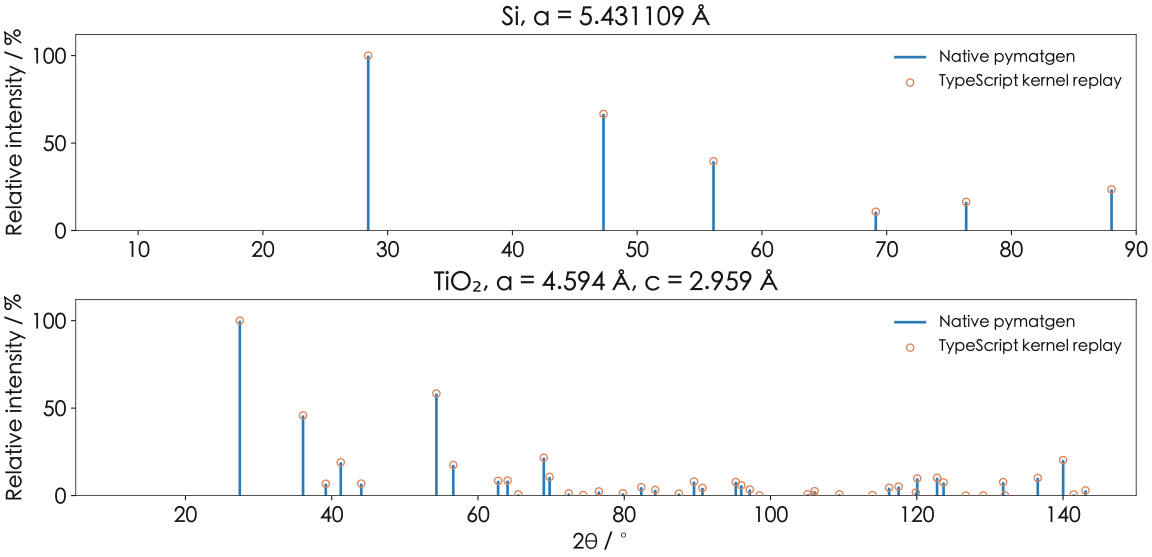
The largest peak across the reference range is normalized to 100. Figure 1 displays calculated discrete reflections of synthetic cells, with heights in relative-intensity units.
Reference inputs and calculation domain
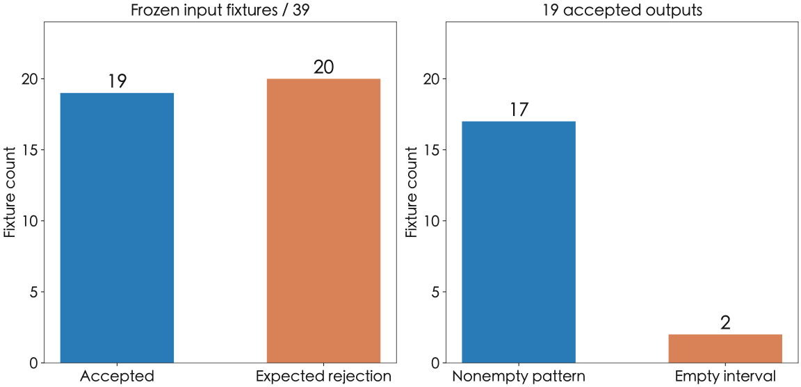
The double-precision TypeScript kernel uses pymatgen 2026.9.23 XRDCalculator as its reference. The 39 frozen inputs comprise 19 accepted results, including two empty peak intervals, and 20 expected rejections. They cover silicon, gold, rutile, hexagonal titanium, a triclinic cell, mixed occupancies, repeated sites, vacancies, wavelength changes and the 200-site limit.
Reflections are filtered by their reciprocal-vector lengths, with Friedel symmetry and reuse of elemental scattering factors reducing repeated work. Peak merging uses 10⁻⁵° bins and ties-to-even rounding, with a 0.001 % intensity cutoff. Enumeration and normalization cover 0–150° before cropping the requested interval. The original lattice, coordinates and occupancies are retained, with symprec=0 by default.
Dense peak tables and boundary cases
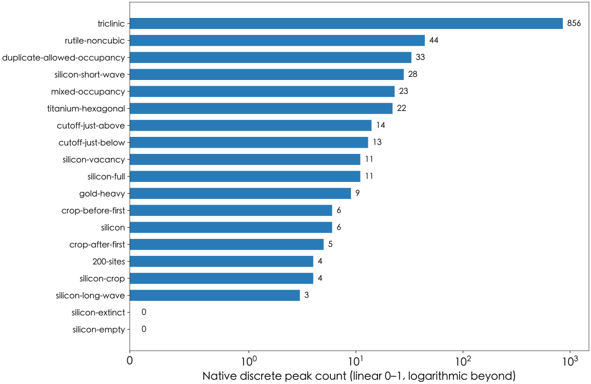
The triclinic fixture contains 856 discrete peaks and tests general reciprocal lattices and family merging. Replay also covers either side of the intensity cutoff, cropping at the first peak and rejection reasons. Each input retains its native peak table, reference timing and SHA-256 identity.
Peak-by-peak numerical agreement
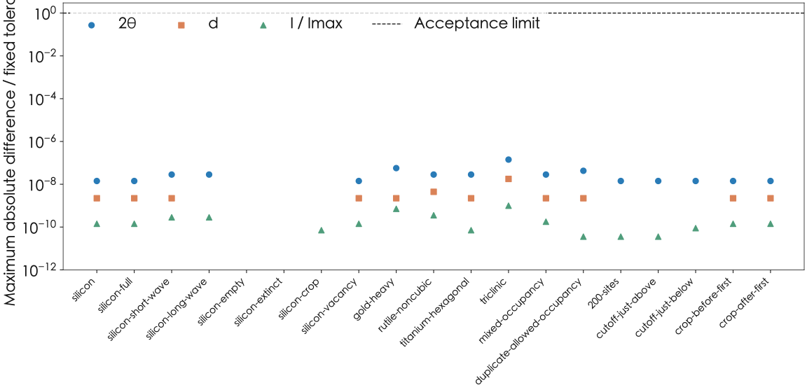
Acceptance compares individual peaks. Peak counts, membership and family sets must agree; , d and relative intensity use the pre-existing absolute tolerances below. The intensity tolerance applies to the 0–100 numerical scale.
| Field | Absolute tolerance | Maximum absolute difference |
|---|---|---|
| 2θ / ° | 1×10⁻⁶ | 1.4211 × 10⁻¹³ |
| d / Å | 1×10⁻⁷ | 1.7764 × 10⁻¹⁵ |
| Relative intensity / 0–100 | 1×10⁻⁴ | 9.9476 × 10⁻¹⁴ |
| Peak membership, hkl families | Exact | All equal |
Across the 19 accepted inputs, maximum differences in angle, spacing and intensity are 1.4211×10⁻¹³°, 1.7764×10⁻¹⁵ Å and 9.9476×10⁻¹⁴. All 39 tests pass, including expected rejections. The plotted differences show that the two double-precision programs give closely matching results for the same structure. The accuracy of the structural parameters depends on their source and measurement conditions.
Product exports additionally contain six calculated peaks for COD 1512541 and 14 for JARVIS dft_3d_JVASP-1002. The maximum angular difference from native pymatgen is 2.8422×10⁻¹⁴° in both cases. Peak tables are calculated from each record’s lattice, atomic coordinates and occupancies, with source identities and input hashes retained. [2, 3, 4]
Paired measurements of the warmed silicon task
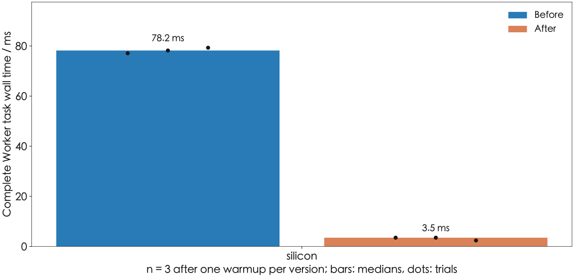
Old and new distribution Workers alternate the silicon fixture in the same macOS Chromium session, with one warmup and three measured trials per version. Old observations are 77.1, 78.2 and 79.3 ms; new observations are 3.5, 3.5 and 2.4 ms. The median falls from 78.2 to 3.5 ms, a 95.5 % reduction and approximately 74.7 ms saved. [5]
| Input | Before / ms | After / ms | Time reduction |
|---|---|---|---|
| silicon | 78.2 | 3.5 | 95.5 % |
Both versions retain all 21 progress events and identical scientific fields; device-self-test time is the sole field removed from comparison. Seventeen current distribution checks cover Worker protocol, storage, domain and numerics. Cancellation takes approximately 1.1 ms and retry succeeds. All 39 frozen fixtures retain their original position, spacing and intensity tolerances.
Timing covers submission, computation, progress notifications and result delivery in a warmed Worker. Reproduction uses identical inputs, initialization state and complete-task boundaries; individual timings determine the plotted median and range.
Historical costs for different inputs
Enumeration cost depends jointly on reciprocal-space candidates and site count. The current domain is an explicit three-dimensionally periodic cell with 1–200 sites, wavelength 0.5–3 Å and angle intervals within 5–150°. The integer box permits up to 250000 candidates and candidates times sites up to 5000000. Large cells can produce dense reciprocal points even with few atoms.
Historical single observations give approximately 1.89 ms for the silicon Node kernel and 9.11 ms for native Python; the 200-site fixture takes approximately 27.89 and 35.31 ms. The table preserves these cost records, with each native and Node timing entry point available in the data.
Product receipts record task times of 0.135 s for COD and 0.081 s for JARVIS. Independent Python verification also includes work such as initialization, so these records measure different processes. The preceding section's paired measurements, from task submission to result transfer, establish the optimization's effect. Historical records describe the cost of different inputs.
| Fixture | Node / ms | Python / ms |
|---|---|---|
| silicon | 1.894 | 9.111 |
| rutile-noncubic | 0.548 | 3.795 |
| triclinic | 4.806 | 8.720 |
| 200-sites | 27.886 | 35.311 |
Structure and experimental conditions
The calculation uses the kinematic approximation, real normal atomic scattering factors and an occupancy-averaged structure. Real scattering factors give equal Friedel-pair intensities; partial site occupancies enter Bragg reflections through coherently averaged amplitudes. The output consists of discrete peaks normalized over the specified range, suitable for structural previews and reference peak-table reproduction. Experimental-pattern modelling additionally considers anomalous scattering, thermal motion, defects and disorder, preferred orientation, line shape, background and instrument response.
VTNA: reaction-order analysis and validation
Concentration normalization and the time axis
Reaction-progress curves usually advance at different rates when initial concentrations change. Variable Time Normalization Analysis (VTNA) rescales time with candidate concentration powers to find reaction orders that bring these curves into alignment. Overlay quality contributes to kinetic interpretation alongside temperature, material balances, catalyst state and experimental design. [6, 7]
For an apparent rate law , continuous normalized time for the selected species is . At fixed powers, experiments sharing a progress function may approach an overlay, provided their conditions and progress definitions are comparable.
The numerical core first computes concentration midpoints, then applies powers and accumulates:
This generally differs from applying powers before trapezoidal integration. Fractional and negative orders and sparse sampling can amplify the difference, making the discrete integration sequence part of the porting comparison.
Time is standardized to s and concentration to M, giving normalized-time units of . Input checks cover time ordering and the domain of concentration powers. Provenance, initial concentrations, temperature, solvent and unit conversions are preserved with the result.
Fitting constraints and selected orders
Curves share the same alignment and concentration scaling; normalized time is scaled consistently before global fitting. Through-origin, polynomial and monotonic constrained polynomial models use all experimental points in the score:
The score is in scaled-concentration units. Measurement uncertainty and statistical likelihood require a separate error model.
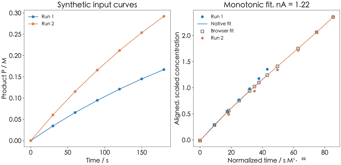
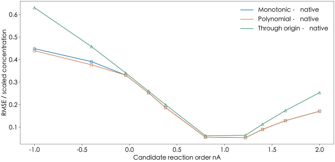
The order search evaluates a coarse grid, refines promising regions and retains scores for all evaluated points. Refitting at the selected order verifies agreement with the search score. For this synthetic input, monotonic and ordinary polynomial fits select 1.22, while through-origin fitting selects 0.80; both implementations make the same selections. The comparison quantifies the influence of fitting constraints on the selected apparent order.
Scores and independent array verification
The frozen reference contains 32 fixtures and solver-path outputs. Field-level comparison covers array lengths, fields, strings, booleans, normalized times, selected orders, score surfaces, fitted curves, residuals and warnings. Solver parameters must agree exactly. [8]
| Item | Rule or result |
|---|---|
| Frozen fixtures | 32 |
| Numbers compared | 13436 |
| Score / RMSE tolerance | 1×10⁻⁷ |
| Other numerical tolerance | 1×10⁻⁹ + 1×10⁻⁷ |native| |
| Maximum absolute difference | 5.150946336129891×10⁻¹¹ |
| Confirmed tied optima | 0 |
| Explicit out-of-domain rejections | 4 |
Scores and overlay RMSE use an absolute tolerance of 10⁻⁷; other numbers use . Selected optima agree throughout this corpus. Across 13436 values, the maximum absolute difference is 5.1509×10⁻¹¹, in a scaled residual of the 500-observation fixture.
The archived probe’s overall status is blocked and the independent field-level verification reports numeric-passed; both records are preserved separately. Four out-of-domain fixtures retain native results and verify the corresponding browser domain limitations. This checks both in-domain fitting and out-of-domain handling.
Two product exports additionally cover 3,610 numerical values, with a maximum difference of 8.8818×10⁻¹⁶. The offline record uses a fully cached runtime and dependencies.
Residuals and order sensitivity
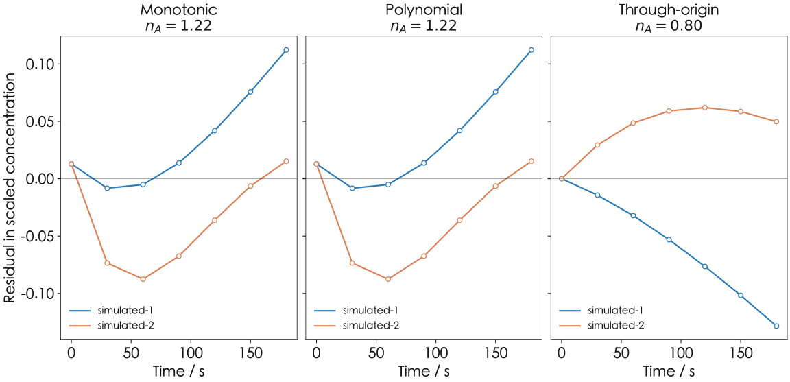
The residual figure makes these effects visible. Changing the fitting method changes the selected order, while native and browser residuals nearly coincide within each method. Pointwise residuals and score curves help distinguish differences caused by fitting assumptions from numerical differences introduced by the port.
The score envelope retains searched points satisfying , describing order sensitivity on the specified grid and threshold. Interpretation also uses the initial-concentration design, confounding caused by jointly varied species, material balance and same-excess information. Statistical confidence intervals require experimental replication and a measurement-error model.
Solver settings and execution costs
The numerical core is pinned to Auto-VTNA 1.2.4 and revision 4acdbd53bc38f33e2ba2fa8f50a7ba3fad93c88d. The browser uses Pyodide 314.0.7, Python 3.14.2, polyfit 1.0, OSQP 1.1.3 and SCS 3.3.1. OSQP retains eps_abs=eps_rel=10⁻⁸; the SCS fallback uses eps=10⁻⁴ and max_iters=100000. Normal execution, fallback, retry and full-chain failure all have retained verification records.
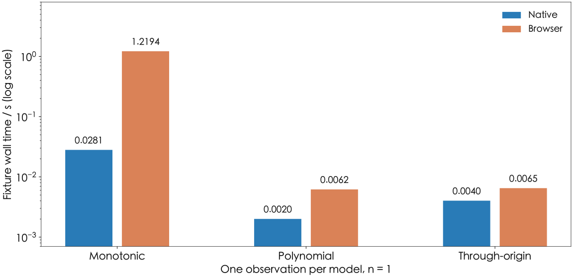
| Fit | Native / s | Browser / s | Selected order |
|---|---|---|---|
| monotonic | 0.028084 | 1.2194 | 1.22 |
| polynomial | 0.002007 | 0.0062 | 1.22 |
| origin | 0.004025 | 0.0065 | 0.80 |
The Python scientific runtime and solvers require about 52.3 MiB of assets. In the Chromium test, runtime loading takes 3.2695 s and all dependencies are ready at 3.2798 s, measured from the same starting point. WASM linear memory is 234749952 bytes, approximately 223.9 MiB. The browser process also uses memory for JavaScript objects and other allocations.
For the same synthetic input, monotonic, polynomial and through-origin browser fits take approximately 1.2194, 0.0062 and 0.0065 s. Figure 9 also shows native times, with one measurement per record. Each fitting path includes different initialization and solver work, so Figure 9 describes the cost of these executions. Comparing repeated performance requires the same initialization state.
Task isolation and cancellation follow the shared execution section. VTNA retains the measured costs of each solver path and runtime loading.
Input domain and kinetic interpretation
The browser domain permits 2–4 experiments, up to 500 observations, 1–2 normalized species, polynomial degrees 1–5 and up to 61 score evaluations, with observations times evaluations capped at 21000 and positive residual degrees of freedom. Tasks have a 120 s wall limit and a 768 MiB admission-memory estimate. Out-of-domain inputs return explicit reasons while grids, refinement and solver settings retain their definitions.
Covarying initial concentrations confound order combinations. Narrow concentration ranges, low signal-to-noise ratios, mixing and mass-transfer control can also produce similar overlays. Catalyst deactivation, product inhibition and reversibility require additional experiments and kinetic models.
Data and reproduction
Saved XRD and VTNA results can be independently verified from the public gzip JSON and CSV files. XRD data contain 39 fixed inputs and native/browser peak tables. Pairing peak membership and families permits separate calculation of differences in , d and relative intensity, together with checks of 19 accepted results and 20 expected rejections. optimization.json and optimization.csv provide warmup markers, individual timings and output-agreement records for recalculating paired silicon-task medians and time reductions.
VTNA data provide original inputs, normalized times, scores, fitted curves and pointwise residuals. Curves are reconstructed using the recorded discrete-integration order, concentration scaling, grid and fitting constraints, then compared with the field-specific tolerances reported here. Repeating XRD uses the pinned pymatgen and scattering coefficients; VTNA uses the pinned Auto-VTNA, numerical dependencies and solver configuration. Public attachments support reproduction of saved arrays, figures and statistics.
Data and sources
- XRD · Raw numerical results and native references · JSON gzip
- XRD · Numerical summary · CSV
- XRD · Provenance and verification records · JSON
- XRD · All discrete peaks · CSV
- XRD · Optimization pairs, builds and cancellation · JSON
- XRD · All optimization timings including warmup · CSV
- XRD · Fixture coverage and peak counts · CSV
- VTNA · Raw numerical results and native references · JSON gzip
- VTNA · Numerical summary · CSV
- VTNA · Provenance and verification records · JSON
- VTNA · Normalized and fitted curves · CSV
- VTNA · Pointwise residuals · CSV
- VTNA · Fit wall times · CSV
- pymatgen: XRDCalculator and powder diffraction model
- Mol2Mat: archived XRD evidence and source identities
- Crystallography Open Database: theoretical Si record 1512541
- NIST JARVIS-DFT: structural data and calculation provenance
- Mol2Mat: paired real-Worker scheduling and state-reuse measurements, 2026-10-10
- D. Dalland, L. Schrecker, K. K. Hii. Auto-VTNA: an automatic VTNA platform for determination of global rate laws. Digital Discovery 3, 2118–2129 (2024). doi:10.1039/D4DD00111G
- J. Burés. Variable Time Normalization Analysis: General Graphical Elucidation of Reaction Orders from Concentration Profiles. Angewandte Chemie International Edition 55, 16084–16087 (2016). doi:10.1002/anie.201609757
- Mol2Mat: frozen VTNA sources, browser arrays and verification
- Auto-VTNA upstream source and usage documentation
- Pyodide: Python scientific runtime for WebAssembly