Running VTNA kinetic analysis in the browser
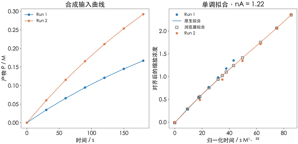
Compiling the Auto-VTNA core and solvers for the browser. Curves, scores and residuals show agreement with native results and how fitting constraints affect the selected orders.
2026-10-03 · Mol2Mat · revision 1
Concentration-curve overlay and numerical reproduction
Reaction-progress curves usually advance at different rates when initial concentrations change. Variable Time Normalization Analysis (VTNA) rescales time with candidate concentration powers to find reaction orders that bring these curves into alignment. Overlay quality contributes to kinetic interpretation alongside temperature, material balances, catalyst state and experimental design.[1,2]
Mol2Mat compiles the Auto-VTNA Python numerical core and optimization solvers into a browser Worker. Preprocessing, discrete integration, order search and fitting constraints follow the original algorithm, as does the fallback sequence when a solver fails. Across 32 fixed tests and 13436 values, the maximum absolute difference between native and browser results is 5.1509×10⁻¹¹.[3]
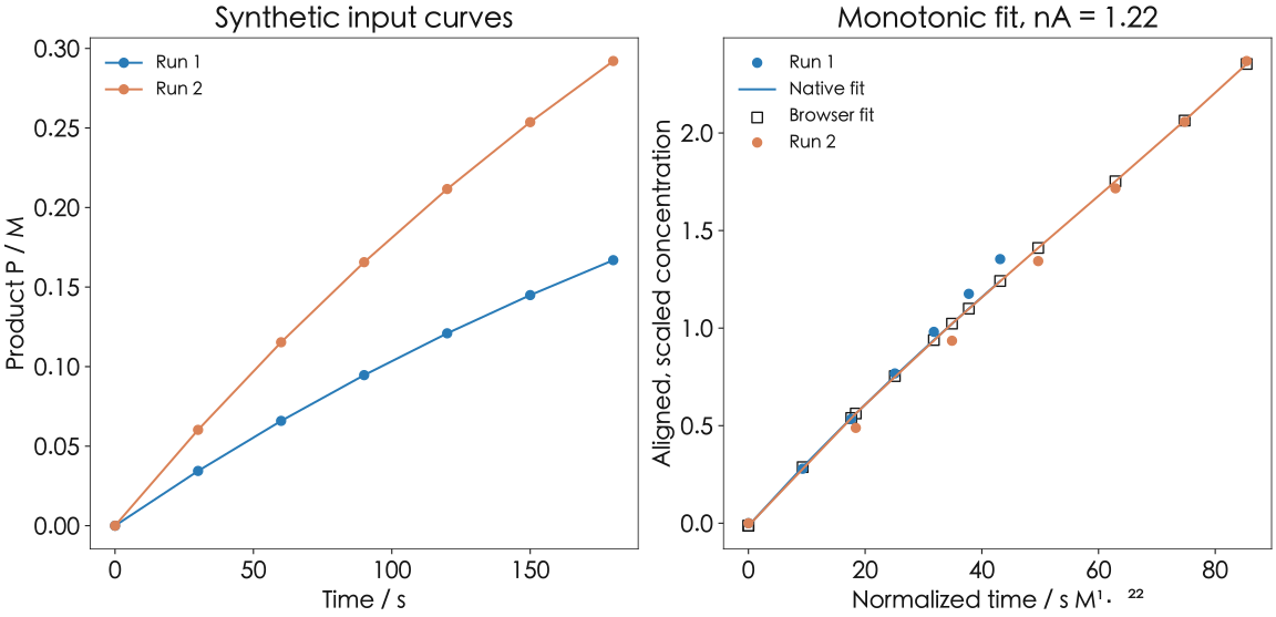
The figures use two synthetic concentration profiles to show time normalization, scores and residuals. Both implementations select the same orders, while changing the fitting constraints changes that choice. This example checks reproduction of the algorithm and shows how fitting assumptions affect kinetic inference.
Rescaling time with concentration
For an apparent rate law , continuous normalized time for the selected species is . At fixed powers, experiments sharing a progress function may approach an overlay, provided their conditions and progress definitions are comparable.
The numerical core first computes concentration midpoints, then applies powers and accumulates:
This generally differs from applying powers before trapezoidal integration. Fractional and negative orders and sparse sampling can amplify the difference, making the discrete integration sequence part of the porting comparison.
Time is standardized to s and concentration to M, giving normalized-time units of . Input checks cover time ordering and the domain of concentration powers. Provenance, initial concentrations, temperature, solvent and unit conversions are preserved with the result.
Fitting constraints affect the selected orders
Curves share the same alignment and concentration scaling; normalized time is scaled consistently before global fitting. Through-origin, polynomial and monotonic constrained polynomial models use all experimental points in the score:
The score is in scaled-concentration units. Measurement uncertainty and statistical likelihood require a separate error model.
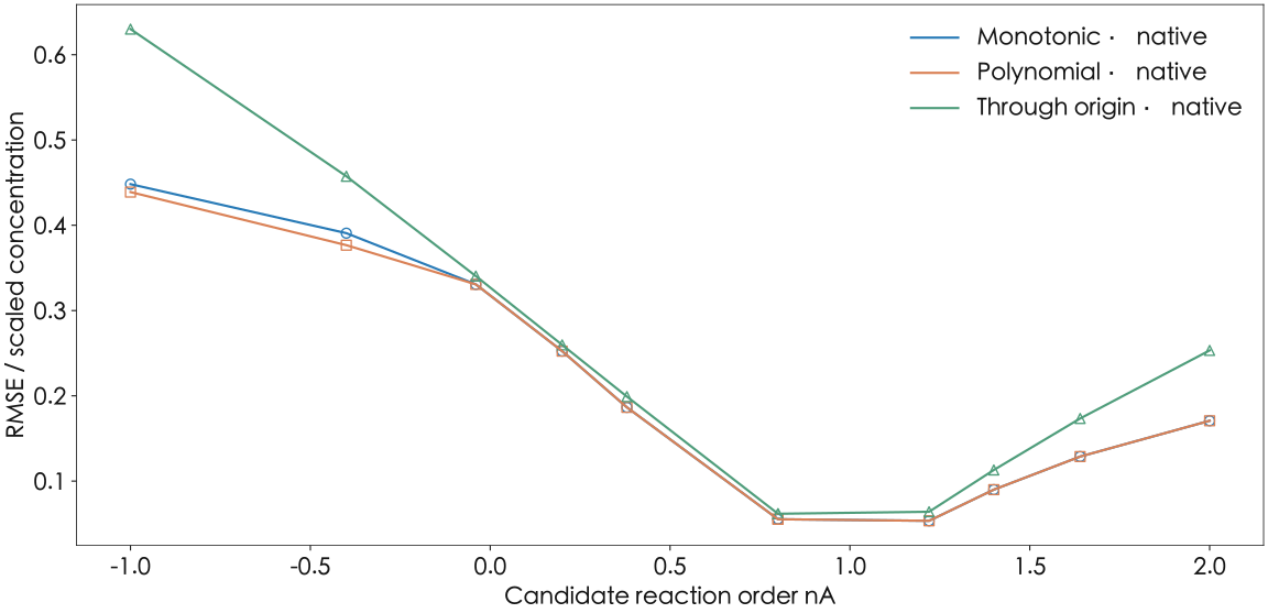
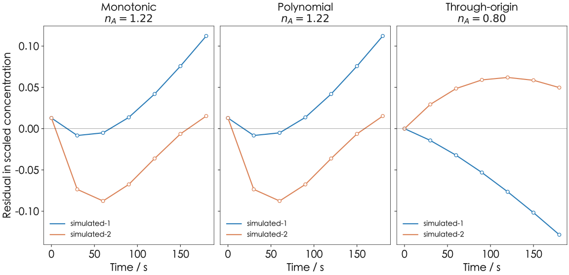
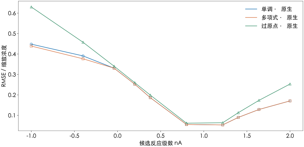
The search evaluates an initial grid, then refines promising regions, saving the score at every order tested. After selecting an order, it refits the curves and checks that the score matches the search result. Monotonic and ordinary polynomial fits select 1.22; through-origin fitting selects 0.80. Native and browser execution make the same choices. Fitting constraints account for the visible differences, while differences between implementations are barely visible in the figure.
The score envelope collects evaluated points satisfying , quantifying order sensitivity under the chosen grid and threshold. Statistical confidence intervals additionally require experimental replication and a measurement-error model. Interpretation combines initial-concentration design rank, covariation of concentrations, material balances and same-excess information.
Browser compilation of the Python core and native solvers
The numerical core pins Auto-VTNA 1.2.4 at revision 4acdbd53bc38f33e2ba2fa8f50a7ba3fad93c88d and ports explore_orders and VTNA_orders. The Mol2Mat input wrapper is also fixed by hash, making the literature method, upstream algorithm and product input layer separately traceable.[1,3]
The browser uses Pyodide 314.0.7, Python 3.14.2, polyfit 1.0, OSQP 1.1.3 and SCS 3.3.1. Native and browser versions of NumPy, SciPy, pandas and cvxpy are recorded separately; numerical arrays provide the cross-environment fidelity check. Optimization retains the OSQP / SCS path, while dependency assets also include Clarabel.
Compiling SCS requires resolving a difference in BLAS calling conventions. The WASM f2c interface differs from the original declarations and calls, requiring changes at 32 locations. The patch handles the ABI; objectives, matrix construction and solver tolerances retain their original definitions. OSQP uses eps_abs = eps_rel = 10⁻⁸; the SCS fallback uses eps = 10⁻⁴ and max_iters = 100000.
Solver validation covers normal OSQP, SCS fallback, SCS retry and complete-chain failure, with explicit fault injection for exceptional paths. Complete failure preserves a failure output. Product-flow checks separately cover Worker asset identity, cancellation and lifecycle.
Field-by-field validation of native and browser outputs
The frozen reference contains 32 fixtures and solver-path outputs. Field-level comparison covers array lengths, fields, strings, booleans, normalized times, selected orders, score surfaces, fitted curves, residuals and warnings. Solver parameters must agree exactly.[3]
Scores and overlay RMSE use an absolute tolerance of 10⁻⁷; other numbers use . Selected optima agree throughout this corpus. Across 13436 values, the maximum absolute difference is 5.1509×10⁻¹¹, in a scaled residual of the 500-observation fixture.
The archived probe’s overall status is blocked and the independent field-level verification reports numeric-passed; both records are preserved separately. Four out-of-domain fixtures retain native results and verify the corresponding browser domain limitations. This checks both in-domain fitting and out-of-domain handling.
Two product exports additionally cover 3610 values with a maximum difference of 8.8818×10⁻¹⁶. The offline flow uses a cached runtime; offline execution requires all necessary assets to be cached.[3]
| Item | Rule or result |
|---|---|
| Frozen fixtures | 32 |
| Numbers compared | 13436 |
| Score / RMSE tolerance | 1×10⁻⁷ |
| Other numerical tolerance | 1×10⁻⁹ + 1×10⁻⁷ |native| |
| Maximum absolute difference | 5.150946336129891×10⁻¹¹ |
| Confirmed tied optima | 0 |
| Explicit out-of-domain rejections | 4 |
Runtime loading, solver timing and memory metrics
The Python scientific runtime and solvers require about 52.3 MiB of assets. In the Chromium test, runtime loading takes 3.2695 s and all dependencies are ready at 3.2798 s, measured from the same starting point. WASM linear memory is 234749952 bytes, approximately 223.9 MiB. The browser process also uses memory for JavaScript objects and other allocations.
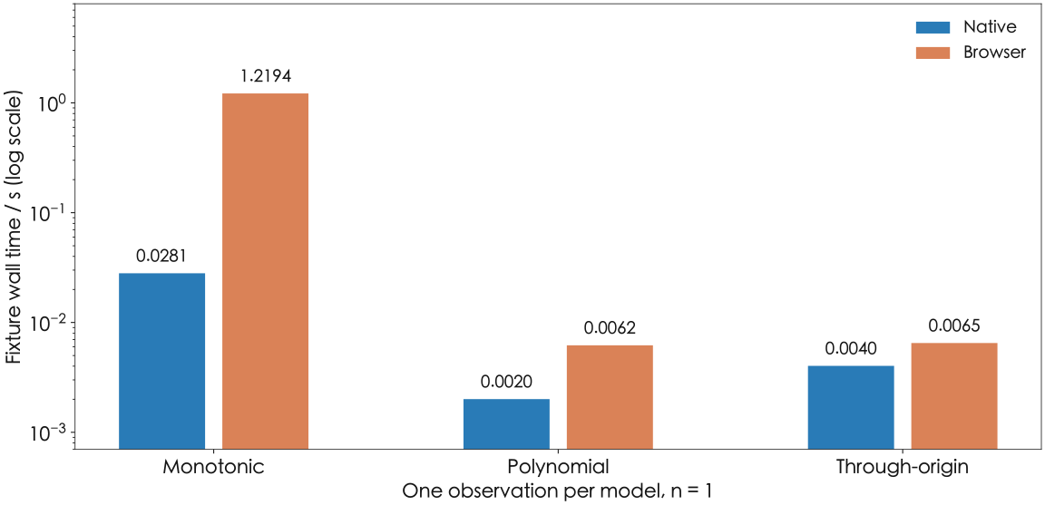
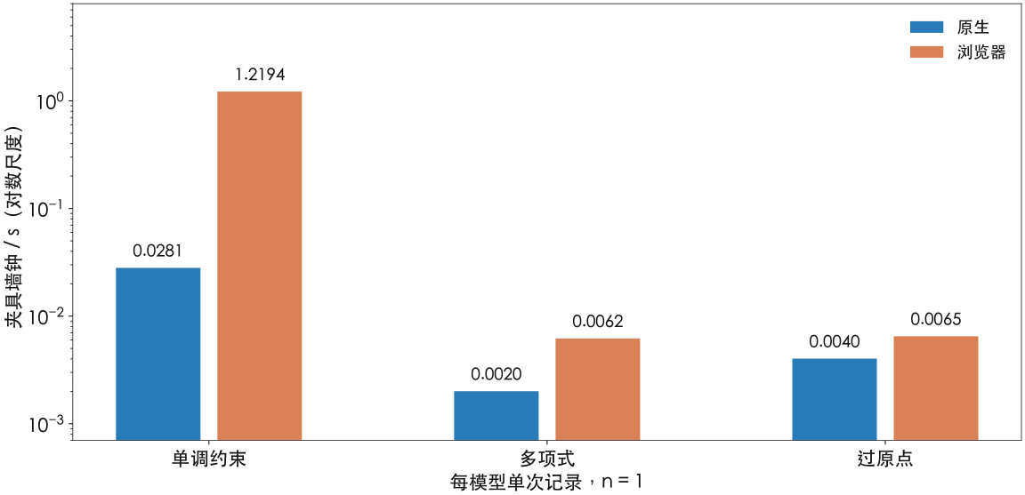
For the same synthetic input, monotonic, polynomial and through-origin browser fits take approximately 1.2194, 0.0062 and 0.0065 s. The figure also shows native times, with one measurement per record. Each fitting path includes different initialization and solver work, so the figure describes the cost of these executions. Comparing repeated performance requires the same initialization state.
The browser domain permits 2–4 experiments, up to 500 observations, 1–2 normalized species, polynomial degrees 1–5 and up to 61 score evaluations, with observations times evaluations capped at 21000 and positive residual degrees of freedom. Tasks have a 120 s wall limit and a 768 MiB admission-memory estimate. Out-of-domain inputs return explicit reasons while grids, refinement and solver settings retain their definitions.
| Fit | Native / s | Browser / s | Selected order |
|---|---|---|---|
| monotonic | 0.028084 | 1.2194 | 1.22 |
| polynomial | 0.002007 | 0.0062 | 1.22 |
| origin | 0.004025 | 0.0065 | 0.80 |
Experimental design and interpreting reaction orders
Covarying initial concentrations confound order combinations. Narrow concentration ranges, low signal-to-noise ratios, mixing and mass-transfer control can also produce similar overlays. Catalyst deactivation, product inhibition and reversibility require additional experiments and kinetic models.
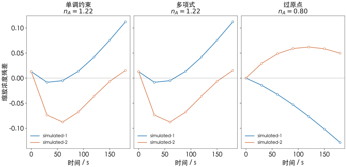
The residual figure makes these effects visible. Changing the fitting method changes the selected order, while native and browser residuals nearly coincide within each method. Pointwise residuals and score curves help distinguish differences caused by fitting assumptions from numerical differences introduced by the port.
The implementation serves VTNA analysis under explicit conditions and bounded data sizes, preserving input observations, candidate orders, score history and diagnostics. Experimental replication, identifiable designs and independent chemical judgement support conclusions about real kinetics.
Frozen inputs, build patches and numerical replay
The bundle contains native inputs and outputs, browser reports, independent verification, curve and summary CSVs, hashes of the core and build scripts, and the SCS ABI patch. Plotted inputs, grid points, fits and residuals are traceable.
After extraction, python replay.py --article vtna checks saved arrays and domain limitations. Repository tools/compute-build/vtna/verify_q5_probe.py additionally checks pinned sources and solver versions. Build notes provide native recomputation entry points, dependency versions and patches.
浏览器端 VTNA 动力学分析与数值一致性验证
将 Auto-VTNA 的数值核心和求解器编译到浏览器,以曲线、评分和残差展示原生对照,以及拟合约束对级数选择的影响。
2026-10-03 · Mol2Mat · revision 1
浓度曲线叠合与数值复现
同一反应在不同初始浓度下,进程曲线通常会以不同速度推进。Variable Time Normalization Analysis(VTNA)用浓度的候选幂次重新缩放时间轴,寻找能让这些曲线叠合的反应级数。叠合程度与温度、物料衡算、催化剂状态和实验设计一起,为动力学解释提供依据。[1,2]
Mol2Mat 将 Auto-VTNA 的 Python 数值核心与优化求解器编译到浏览器 Worker。预处理、离散积分、级数搜索和拟合约束沿用原算法,求解器失败时也按相同顺序回退。32 个固定测试包含 13436 个数值,原生与浏览器结果的最大绝对差为 5.1509×10⁻¹¹。[3]
下面用两组合成浓度曲线展示时间归一化、评分和残差。两套程序选出相同级数,而改变拟合约束会改变这一选择。这组例子既能检查程序是否复现原算法,也能看到拟合假设如何影响动力学推断。
浓度归一化改变时间轴
对表观速率 ,指定归一化物种的连续时间为 。在固定浓度幂下,具有共同进程函数的实验可能接近叠合;各实验需采用可比较的条件和同一进程定义。
数值核心先计算浓度中点,再取幂并累加:
这一规则与“先取幂、再作梯形积分”通常给出不同结果。分数幂、负级数与稀疏采样会放大差异,因此离散积分顺序是移植对照的一部分。
时间统一为 s、浓度统一为 M,归一化时间的单位为 。输入检查覆盖时间顺序及浓度幂的定义域;来源、初始浓度、温度、溶剂与单位转换随结果保存。
拟合约束影响级数选择
每组曲线按相同规则对齐并缩放浓度,归一化时间在全局拟合前统一缩放。拟合可选择过原点、多项式或单调约束多项式,全部实验点共同参与评分:
该评分的单位为缩放浓度,测量不确定度与统计似然需另行指定误差模型。
搜索先评价粗网格,再细化较优区域,保存每个级数对应的评分。选定级数后重新拟合曲线,核查其评分与搜索时一致。图中,单调和普通多项式拟合都选择 1.22,过原点拟合选择 0.80;原生与浏览器得到相同结果。差别来自拟合约束,而两套实现间的差别在图上几乎不可见。
score envelope 收集满足 的已搜索点,量化指定网格和阈值下的级数敏感性。统计置信区间则需要实验重复与测量误差模型。初始浓度设计秩、共同变化引起的级数混淆、物料衡算与 same-excess 信息共同参与解释。
Python 核心与原生求解器的浏览器编译
数值核心固定 Auto-VTNA 1.2.4 来源和仓库修订 4acdbd53bc38f33e2ba2fa8f50a7ba3fad93c88d,移植 explore_orders 与 VTNA_orders。Mol2Mat 的输入封装也以哈希固定,使文献方法、上游算法和产品输入层分别可追溯。[1,3]
浏览器使用 Pyodide 314.0.7、Python 3.14.2,以及 polyfit 1.0、OSQP 1.1.3 和 SCS 3.3.1。原生与浏览器的 NumPy、SciPy、pandas、cvxpy 版本分别记录,数值数组承担跨环境一致性检查。优化路径沿用 OSQP / SCS;依赖资产另包含 Clarabel。
SCS 的编译需要解决 BLAS 调用约定的差异。WASM 使用的 f2c 接口与原声明和调用方式不同,因而调整了 32 处接口代码。补丁只处理 ABI,优化目标、矩阵构造和求解器容差沿用原定义:OSQP 的 eps_abs = eps_rel = 10⁻⁸;SCS 回退的 eps = 10⁻⁴、max_iters = 100000。
求解链验证覆盖正常 OSQP、SCS 回退、SCS 重试和全链失败,使用明确故障注入检查异常路径。全链失败保留失败输出。Worker 的资源身份、取消和生命周期另由产品流程验证。
原生输出与浏览器数组的逐项验证
固定参考包含 32 个夹具及求解器路径输出。逐项比较数组长度、字段、字符串、布尔值、归一化时间、最优级数、评分曲面、拟合曲线、残差和警告;求解器参数要求精确一致。[3]
评分与叠合 RMSE 使用 10⁻⁷ 绝对容差,其他数值采用 。本组最优点一致,13436 个数值的最大绝对差为 5.1509×10⁻¹¹,来自 500 观测夹具的缩放残差。
归档探针的总体状态为 blocked,独立逐字段验证状态为 numeric-passed,两项记录分别保留。四个超域夹具保存原生结果,并核查浏览器返回对应域限制。这样同时检验范围内的拟合结果与范围外的处理规则。
两个产品导出还覆盖 3610 个数值,最大差为 8.8818×10⁻¹⁶;其中离线流程使用已缓存运行时。离线执行的前提是所需资产完整缓存。[3]
| 项目 | 比较规则或结果 |
|---|---|
| 固定夹具 | 32 |
| 比较数值 | 13436 |
| 评分 / RMSE 容差 | 1×10⁻⁷ |
| 其他数值容差 | 1×10⁻⁹ + 1×10⁻⁷ |native| |
| 最大绝对差 | 5.150946336129891×10⁻¹¹ |
| 确认并列最优点 | 0 |
| 显式域外拒绝 | 4 |
运行时装载、求解耗时与内存指标
Python 科学运行时与求解器资源约 52.3 MiB。Chromium 测试中,装载运行时用了 3.2695 s,全部依赖在 3.2798 s 时就绪,两个时间从同一起点计量。WASM 线性内存为 234749952 字节,约 223.9 MiB;浏览器进程还会使用内存保存 JavaScript 对象等内容。
对同一组合成输入,浏览器的单调、多项式和过原点拟合分别约用 1.2194 s、0.0062 s 和 0.0065 s。图中同时给出原生耗时,每条记录均测量一次。各拟合路径包含的初始化和求解工作不同,因此这张图呈现的是此次执行的成本;比较重复运行性能时,需要保持相同的初始化状态。
浏览器域允许 2–4 组实验、最多 500 个观测、1–2 个归一化物种、1–5 阶多项式和最多 61 个评分评价,观测数与评分数乘积最多 21000,拟合须有正残差自由度。任务墙钟上限为 120 s,准入内存估算为 768 MiB。超域输入返回明确原因,网格、细化与求解器设置保持原定义。
| 拟合模型 | Native / s | Browser / s | 选择级数 |
|---|---|---|---|
| monotonic | 0.028084 | 1.2194 | 1.22 |
| polynomial | 0.002007 | 0.0062 | 1.22 |
| origin | 0.004025 | 0.0065 | 0.80 |
实验设计与级数解释
初始浓度共同变化会混淆不同级数组合。狭窄浓度范围、低信噪比、混合与传质控制也可能形成相似叠合。催化剂失活、产物抑制与可逆性需要补充实验与动力学模型。
残差图能直接显示这些影响:不同拟合方式选出的级数发生变化,同一拟合方式下原生与浏览器的残差却几乎重合。结合逐点残差和评分曲线,可以分辨拟合假设带来的偏差与程序移植带来的数值差异。
当前实现适用于明确条件与有限数据规模下的 VTNA 分析,保留输入数据、候选级数、评分历史和诊断信息。实验重复、设计可辨识性及独立化学判断为真实动力学结论提供支撑。
固定输入、构建补丁与数值回放
数据包包含原生输入和输出、浏览器报告、独立验证、曲线与汇总 CSV、数值核心及构建脚本哈希,另附 SCS ABI 补丁。绘图所用输入、网格、拟合和残差均可追溯。
解压后运行 python replay.py --article vtna 可检查保存数组和域限制。仓库 tools/compute-build/vtna/verify_q5_probe.py 进一步核查固定来源及求解器版本;原生重算入口、依赖版本和补丁由构建说明提供。
Data and sources
- Raw numerical results and native references · JSON gzip
- Numerical summary · CSV
- Provenance and verification records · JSON
- Data, replay script and checksum manifest · tar.gz
- Normalized and fitted curves · CSV
- Pointwise residuals · CSV
- Fit wall times · CSV
- Dalland, Schrecker and Hii. Auto-VTNA: an automatic VTNA platform for determination of global rate laws. Digital Discovery (2024).
- Burés. Variable Time Normalization Analysis: General Graphical Elucidation of Reaction Orders from Concentration Profiles. Angewandte Chemie (2016).
- Mol2Mat: frozen VTNA sources, browser arrays and verification
- Auto-VTNA upstream source and usage documentation
- Pyodide: Python scientific runtime for WebAssembly