First-Principles Electron–Phonon Coupling Across the Full Brillouin Zone
A complete three-dimensional silicon k/q representation: 406 regression queries, 19 independent electronic-k queries and 16 independent joint k/q queries, tested against direct first-principles references.
Felix Fei
2026-10-20 · Mol2Mat · revision 2
A silicon research milestone
The calculation is now available in the Mol2Mat browser workspace.
An electron–phonon calculation connects three objects: an electronic state at , a lattice vibration at , and a second electronic state at . Computing each object accurately is only part of the problem. Their phases, normalization, symmetries and numerical representations must remain consistent when they are combined—and when the calculation moves away from the points used to construct the model.
We have completed this chain for diamond silicon in Mol2Mat’s four-valence-band research model. Starting from self-consistent density-functional theory, the implementation constructs phonon dynamical matrices and complex electron–phonon vertices on complete 8 × 8 × 8 electronic and phonon meshes, then evaluates them at continuous coordinates by Fourier interpolation.
The final model passes all 406 existing regression queries, all 19 independent electronic- queries, and all 16 independent joint queries under the original 5 % EPC criterion. The largest errors in these three panels are 4.2691 %, 3.4066 % and 4.5619 %, respectively. The independent predictions were frozen before their direct references were generated; the model remained unchanged throughout those evaluations.
This result establishes a reproducible first-principles EPC calculation across three-dimensional momentum space for the specified silicon model. The calculation preserves the full ultrasoft-pseudopotential vertex, identifies the interpolation resolution required by the response, and validates weak coupling channels individually.
From electronic structure to a complex scattering amplitude
The electronic calculation uses PBE and the GBRV silicon ultrasoft pseudopotential [1, 2], with wavefunction and density cutoffs of 20 and 100 Ha. The diamond primitive cell contains two atoms, giving six Cartesian displacement coordinates. The electronic subspace contains four occupied valence bands, represented by four Wannier functions; the calculation is non-spin-polarized and uses a silicon mass of 28.085 u.
For a Cartesian perturbation of atom along direction , we retain a complex 4 × 4 derivative matrix, written here as . Its units are Ha bohr⁻¹. After diagonalizing the mass-weighted dynamical matrix, the phonon polarization and zero-point displacement convert this derivative into a mode-resolved coupling:
Here and label the electronic basis used for the matrix, and labels the phonon mode. The stored vertex uses the Wannier basis. Unitary transformations at the initial and final electronic endpoints give the corresponding Bloch-band matrix. Keeping the unweighted Cartesian vertex separate from the phonon contraction makes both interpolation and error attribution much clearer.
The final tensor has shape (512, 512, 6, 4, 4): initial , phonon , displacement coordinate, final Wannier index and initial Wannier index. It contains 262,144 combinations and 25,165,824 complex derivative entries, accompanied by 512 complex 6 × 6 dynamical matrices. The two meshes specify interpolation resolution. The self-consistent electronic integration uses its own separately recorded quadrature.
This separation follows the physical organization of EPC calculations. EPW [3] uses localized representations to interpolate electronic, vibrational and coupling quantities onto fine momentum grids. Perturbo [4] connects such first-principles matrix elements to transport and carrier dynamics. In Mol2Mat, the present milestone is the construction and independent numerical validation of the underlying silicon coupling model, implemented through finite-displacement JDFTx responses and explicit operator projection.
Preserving the ultrasoft vertex
With an ultrasoft pseudopotential, the electronic eigenproblem contains an overlap operator:
Atomic displacement changes both and . The response includes the local self-consistent potential, nonlocal projectors, augmentation terms and the transport of the electronic basis. The two electronic endpoints also carry different Bloch phases. Each contribution must use the same reference convention before the positive and negative displacements are differenced.
The implementation saves the projected matrices , , , , and . In its stored operator convention, the centered, transported matrix is
The potential means fix the energy-zero convention, while supplies the two-sided transport correction. Before assembly, the code checks the stored identity , along with the reference Hamiltonian and overlap identities. The native projection operates on saved self-consistent potentials, so evaluating additional electronic endpoints can reuse a converged response.
Central differences normally use displacements of ±0.02 bohr along each selected unit direction. Primitive electronic states embedded in an N-cell supercell carry a factor at each endpoint. The assembled derivative consequently restores the factor when differencing the projected blocks. This normalization matters particularly when combining differently shaped supercells.
Space-group transport acts on all parts of the response together: Cartesian directions, atom permutations, lattice offsets and both electronic endpoint rotations. Reciprocal-boundary relabeling is similarly part of the operator definition. A coordinate crossing a Brillouin-zone boundary must induce the corresponding plane-wave G relabeling; preserving only its wrapped numerical coordinate is insufficient.
These details give the model a consistent complex amplitude. A scalar coupling strength alone would discard the phase and channel information needed to check that consistency.
Identifying the resolution the response actually needs
The route to the final model involved a useful distinction between an accurate numerical reconstruction and a sufficiently expressive physical representation.
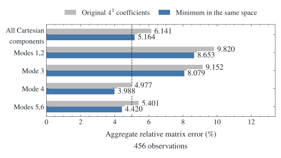
An early 4³ electronic Wannier–Fourier representation reproduced its 64 construction points to numerical precision. At other saved points, however, it showed substantial errors. We therefore asked a sharper question: could any coefficients in the same fixed Fourier space reproduce the available response accurately enough?
For each electronic matrix pair, let evaluate the fixed 64-function basis at 456 saved observations, contain their direct response, and project onto the column space of . The residual separates orthogonally:
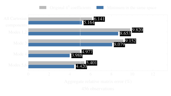
The first term is outside the chosen representation. Changing coefficients within that space cannot remove it. Thin-QR projection gave a minimum aggregate relative error of 5.1642 % for the complete Cartesian vertex and 8.6529 % for the lowest acoustic mode group. Both exceed 5 %. Since pointwise errors bounded by 5 % would also bound their aggregate Frobenius ratio by 5 %, the fixed representation could not satisfy that condition on all 456 observations.
A separate finite-displacement control tested whether inaccurate direct references explained a large historical error. At the audited point, halving the displacement from 0.02 to 0.01 bohr changed the problematic mode’s reference matrix by 0.02742 %. The frozen prediction’s error changed from 21.3081 % to 21.2993 %. That matched control directed the next work toward representation and sampling.
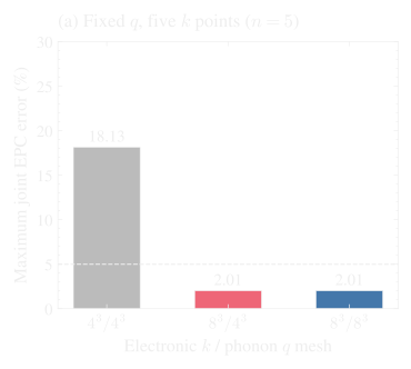
Increasing the electronic mesh to 8³ then reduced the worst error on five fixed- regression queries from 18.1314 % to 2.0051 %. All 392 additional fixed- regression points also passed, with a maximum of 4.2691 %.
The phonon-wavevector direction still required its own resolution. With k8 × q4, eight nonaxial queries at = (2,3,5)/12 retained a worst error of 14.7329 %. After completing q8, the same queries reached 3.6755 %. An axial = (1/3,0,0) query improved from 24.1940 % to 3.2333 %. All coordinates here are fractional coordinates of the primitive reciprocal lattice.
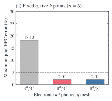
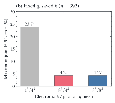
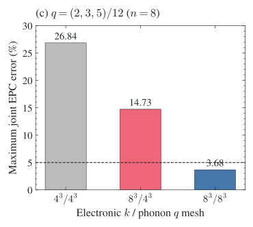
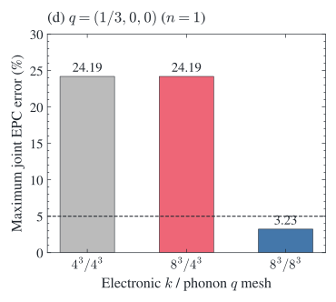
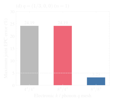
The progression provides a concrete answer to the computational difficulty. Electronic- resolution and phonon- resolution constrain different parts of the same amplitude. Improving one coordinate space can leave the other as the dominant error source.
Completing q8 with 33 additional self-consistent responses
The q8 extension reused the existing q4 responses and axial data. Twelve eight-cell response families supplied the additional nonaxial information; a retained 24-cell axial family supplied another 16 nodes. Together with symmetry, these sources completed all 512 nodes: 64 retained q4 nodes, 16 axial nodes and 432 additional nodes.
The initial signed-displacement plan contained 36 SCF states. Crystal symmetry reduced the required new calculations to 33 by mapping three negative-displacement states to their positive partners. Those operations were checked against the actual atom mapping, weighted electronic integration mesh and FFT grid. The saved positive response could then generate its partner through the certified transformation.
All 33 self-consistent calculations completed. Their inputs each contain 16 atoms, 32 electronic bands and 432 explicitly weighted electronic integration points. The convergence rule required the original 10⁻⁹ SCF residual threshold for two consecutive cycles. The additional eight SCF calculations used later for independent joint validation were a separate reference campaign.
The assembled Cartesian vertex is Fourier transformed over the six momentum-grid axes. Continuous queries evaluate the resulting real-space coefficients with phase factors for both and :
In the implementation, the phase factors average equivalent nearest periodic images. Electronic image selection depends on the difference between Wannier centers; response-image selection depends on the atom position relative to the final Wannier center. The lattice metric determines which images are nearest. These fixed rules preserve the coarse-grid phase identities while specifying the interpolation between nodes. Dynamical matrices use the corresponding atom-centered -space construction.
A subtle symmetry issue emerged during phonon assembly. Very small numerical splitting of a degenerate mode could prevent the original mode-group comparator from finding an equal-dimensional match. The repair enforced the crystal’s little-group symmetry directly on each new dynamical matrix. After Hermitianization, a Reynolds average applies all operations leaving invariant:
The atom-displacement representation includes the lattice-offset phases. Across 84 checked points, the largest relative matrix correction was 0.02246 %, and the largest covariance residual was 3.22 × 10⁻¹⁶. All common-point group dimensions matched. The original q4 values were retained exactly, and the original grouping tolerance remained fixed.
Symmetry reduces the number of response calculations and restores the degeneracies required for mode-resolved comparisons.
Testing predictions before opening the references
The final evaluation separates three questions.
Existing regression. The 406 queries comprise 392 saved fixed- electronic points, five additional fixed- controls, eight nonaxial joint queries and one axial off-grid query. Their direct results were already known during development. All 406 pass with the final q8 model.
Independent electronic . Nineteen new electronic queries were checked against previously exposed symmetry orbits, including crystal operations, time reversal and reverse scattering. Predictions were frozen before the new direct projections were assembled. Their values lie on existing phonon nodes, so this panel tests interpolation at new electronic endpoints. All 19 pass.
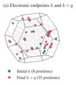
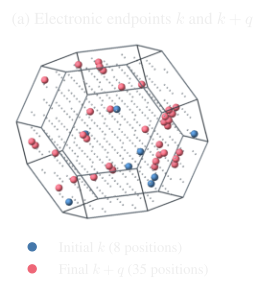
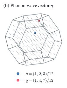
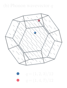
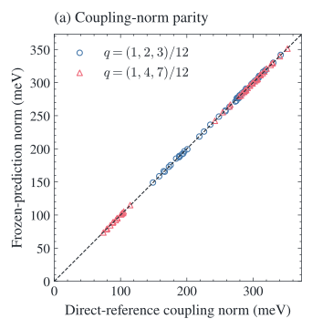
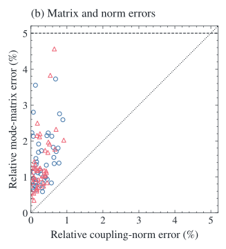
Independent joint . Sixteen queries cover two nonaxial phonon families, = (1,2,3)/12 and = (1,4,7)/12, with eight electronic queries in each. Eight new signed SCF responses supplied the independent references. The independent references were constructed from 208 fixed-potential projection blocks. All 16 pass against the predictions frozen before reference generation.
The model tensor, Fourier rules and 5 % threshold remained fixed. Common-source comparisons checked the new reference assembly against existing sources using a separate 0.5 % criterion.
| Evaluation panel | Queries passing | Maximum electronic-only error | Maximum phonon-only error | Maximum joint error |
|---|---|---|---|---|
| Existing regression | 406 / 406 | 4.2691 % | 0.6853 % | 4.2691 % |
| Independent electronic | 19 / 19 | 3.4066 % | 0.00001261 % | 3.4066 % |
| Independent joint | 16 / 16 | 4.5619 % | 1.9479 % | 4.5619 % |
For the electronic-only comparison, the predicted vertex is paired with the reference dynamical matrix. The phonon-only comparison combines the reference vertex with the predicted dynamical matrix. The joint comparison uses both predictions. These are controlled substitutions into the same coupling calculation; their errors are not additive.
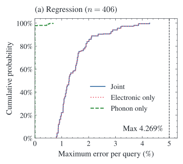
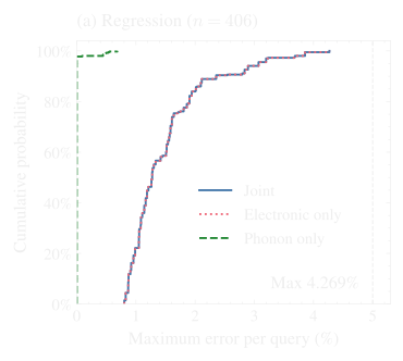
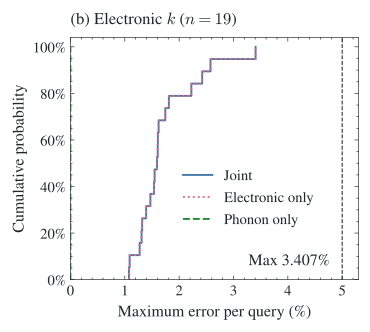
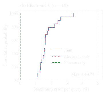
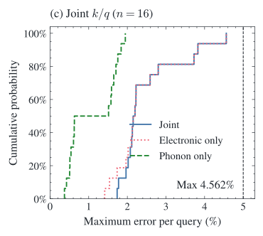
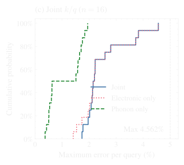
The result combines broad regression coverage with 35 prospective independent queries. Full-BZ describes the continuous three-dimensional representation; numerical accuracy is measured on these explicitly defined test sets.
Validation of weak coupling channels
A single EPC norm is an incomplete validation target. Two complex matrices can have almost the same norm while differing in their orientation in electronic-channel space. A small acoustic response can also arise from cancellation between much larger atomic contributions, amplifying relative errors in the final mode.
Our comparator therefore retains the complete raw vertex and examines individual phonon mode groups. It compares common-gauge matrix differences, coupling norms and singular-value spectra. Within a degenerate group, stacked mode matrices give a channel spectrum that is invariant under unitary mixing of the mode basis. Predicted and reference phonon subspaces are matched through an equal-dimensional bijection maximizing overlap, and coupling norms and channel spectra are also evaluated using each calculation’s own modes.
For example, the common-gauge matrix error is
The point score is the maximum over the full-vertex error and the applicable mode-group matrix, norm and channel-spectrum errors. A missing valid mode match prevents a pass. Zero or unstable modes retain their signed eigenvalues and diagnostic status rather than receiving an artificial positive frequency.
The worst independent joint query occurs at = (1,2,3)/12 and = (1,4,7)/12. Its weakest-mode direct coupling norm is 74.1102 meV, compared with 73.6286 meV for the prediction. That is a norm error of only 0.6498 %. The complex matrix error is 4.5619 %, and the channel-spectrum error is 2.1769 %. This mode carries only 0.5431 % of the squared raw Cartesian-vertex norm. Its atomic cancellation ratio—net mode amplitude divided by the sum of the two atomic amplitudes—is 0.1333.
A plot of total strengths would give this demanding mode little weight. The mode-resolved comparison makes it central to the reported accuracy.
The phonon patterns at this query provide a complementary real-space view. The lowest-mode frequencies are 4.6445 THz for the direct calculation and 4.6260 THz for the frozen prediction. Their squared eigenvector overlap is 0.999994. The close agreement of the vibrational patterns, together with the component-wise scores, places the larger remaining error in the electronic vertex.
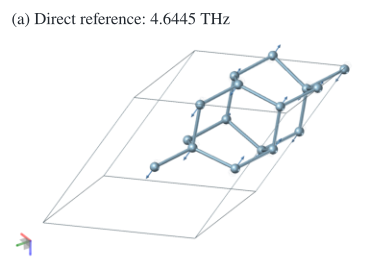
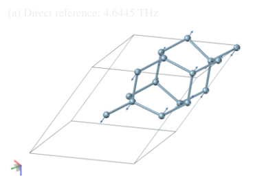
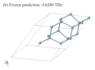
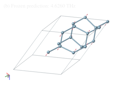
The accompanying interactive three-dimensional view supports rotation, all six mode selections, phase changes, and PNG/GLB export.
These tests target the matrix elements that enter later scattering calculations. Observable convergence will additionally depend on the electronic energy window, phase-space integration, occupations and treatment of energy conservation. Retaining the full complex vertex gives those future calculations a much stronger starting point than a fitted scalar summary.
Eight-core parallel performance
The silicon EPC calculations used an eight-core budget. Independent self-consistent responses and fixed-potential projections can run in parallel. A saved self-consistent potential can also serve new electronic endpoints, reducing repeated calculations.
We compared two core allocations on the same machine. Each configuration advanced the same eight saved SCF states through two further cycles, with elapsed time including startup, checkpoint saving and result output:
| Configuration | Elapsed time | Peak aggregate resident memory |
|---|---|---|
| Four processes × two threads | 704.67 s | 5.03 GiB |
| Eight processes × one thread | 579.69 s | 9.59 GiB |
Eight single-threaded tasks reduced total elapsed time by 17.74 %, while peak memory increased from 5.03 GiB to 9.59 GiB. The final-energy spread between the configurations was 1.28 × 10⁻¹³ Ha. For this workload, sufficient memory allows more independent tasks to run at once and reduces the waiting time.
Thread allocation follows the number of remaining tasks: up to eight single-threaded tasks run concurrently, followed by two threads per task when four or three remain, four threads when two remain, and eight threads for the final task. This keeps available cores in use as the batch approaches completion.
Continuous momentum queries and further calculations
The model supports vertex, phonon-mode and mode-resolved coupling queries at continuous three-dimensional coordinates. Researchers can inspect individual scattering channels, compare predictions with direct references and reproduce errors from the saved matrices. The recorded 441-query interpolation replay reproduced the frozen predictions with a maximum relative difference of 9.86 × 10⁻¹⁶.
The same frozen model is now integrated into the browser’s FP64 WASM computation workflow. Users can evaluate continuous queries, inspect the resulting modes and couplings, compare wavevectors and export the complex matrices. Further work will assess external matrix comparisons, systematic mesh convergence and larger electronic subspaces, supporting subsequent calculations of scattering rates and transport properties from the vertices.
Using the browser workspace
Select electron–phonon coupling in DFT single-point calculation, then enter the electronic wavevector and phonon wavevector in primitive reciprocal fractional coordinates. The workspace compares coupling strengths across all six vibrational modes and between wavevectors. Selecting a mode updates the lattice-vibration animation. The full complex coupling matrices are available in the details panel and can be exported.
The browser uses the silicon model constructed on the 8³ electronic and phonon meshes described above. The first use downloads approximately 384.5 MiB of model data and verifies each file’s size and SHA-256. Subsequent queries run locally through a WebAssembly kernel compiled from C. The kernel evaluates the complex Fourier interpolation in double precision (FP64) and reuses intermediate results for repeated queries at the same . A dedicated Worker runs the calculation while the page remains responsive.
The interpolated complex vertices and dynamical matrices yield phonon frequencies, atomic displacements and mode-resolved couplings. For degenerate modes, the workspace also reports the Frobenius norm of the group coupling matrix to support comparisons between wavevectors. Exported results include the complete complex matrices and the model and kernel versions.
We ran this implementation in Chrome 149 and compared its outputs with the NumPy reference for all 441 queries. The maximum relative differences were 2.11 × 10⁻¹⁵ for the raw vertex and 1.43 × 10⁻¹⁵ for the dynamical matrix; phonon frequencies and group norms were also checked against the same reference. Against the direct first-principles results, all 406 regression queries, 19 independent electronic queries and 16 independent joint queries passed the original 5 % criterion. Detailed results are provided in the browser calculation verification summary.
Accompanying data
The accompanying tables contain all 441 query scores, 96 independent joint mode-group comparisons, matched grid comparisons, and the fixed-representation bounds. The browser WASM verification summary records the 441-query port validation. Figures are supplied in SVG, PDF and PNG formats.
Data and sources
- Browser WASM verification summary
- All 441 query scores
- Independent joint mode-group comparisons
- Matched grid comparisons
- Fixed-representation error bounds
- R. Sundararaman et al. JDFTx: Software for joint density-functional theory. SoftwareX 6, 278–284 (2017). doi:10.1016/j.softx.2017.10.006
- K. F. Garrity et al. Pseudopotentials for high-throughput DFT calculations. Computational Materials Science 81, 446–452 (2014). doi:10.1016/j.commatsci.2013.08.053
- H. Lee et al. Electron–phonon physics from first principles using the EPW code. npj Computational Materials 9, 156 (2023). doi:10.1038/s41524-023-01107-3
- J.-J. Zhou et al. Perturbo: A software package for ab initio electron–phonon interactions, charge transport and ultrafast dynamics. Computer Physics Communications 264, 107970 (2021). doi:10.1016/j.cpc.2021.107970