Implementation and numerical validation of browser-local JDFTx DFT
A browser implementation of double-precision plane-wave JDFTx: native comparisons for six fixed systems, atomic and Al cell relaxation, energy-derivative checks, and conditions for data verification and computational reproduction.
Felix Fei
2026-10-12 · Mol2Mat · revision 1
Abstract
Plane-wave pseudopotential density-functional theory describes electronic structure, atomic forces and cell stress within a common framework for molecules and periodic materials. Mol2Mat implements JDFTx in double precision in the browser, including electronic self-consistency, atomic relaxation and cell relaxation. The comparisons use H₂O, NH₄⁺, diamond Si, rocksalt MgO, face-centered cubic (fcc) Al and spin-polarized body-centered cubic (bcc) Fe. These systems span neutral and charged molecules, covalent and ionic crystals, metals and spin degrees of freedom. Matched native calculations provide reference energies, forces, stresses and relaxation trajectories.
Six native/browser comparisons contain 28 paired output frames. Each frame is checked for atom identity, cell, energy decomposition, forces, stress, electron count, occupations and occupied eigenvalues. Maximum differences are Ha for total/internal/free-energy quantities, Ha bohr⁻¹ for force components and Ha bohr⁻³ for stress components. H₂O, NH₄⁺, Si and MgO complete fixed-cell atomic relaxation. Al completes cell relaxation and passes its endpoint cell to a new execution instance for an independent single-point check.
Computational configurations from molecules to metals
A plane-wave expansion places molecules and crystals in a common electronic-structure framework. Periodic systems use Bloch wavefunctions; in atomic units, the kinetic-energy cutoff selects reciprocal-space basis components:
These calculations use the PBE exchange-correlation functional, SG15 ONCV pseudopotentials for molecules and GBRV ultrasoft pseudopotentials for periodic crystals. The original JDFTx, SG15 and GBRV methods are sources 1–3 below.
H₂O and NH₄⁺ occupy explicit isolated cells of 18 and 20 bohr, respectively, using truncated Coulomb interactions for finite systems. NH₄⁺ has physical charge +1 and eight valence electrons; coordinates, charge, embedding center and pseudopotentials are fixed with the input. Finite-grid density integrals and near-boundary shell integrals additionally check charge localization. Periodic systems fix the primitive cell, fractional coordinates and mesh, retaining weights for every point and spin channel.
The table lists the computational conditions for the six system classes. Every electronic SCF block requires two consecutive final density residuals below . Atomic relaxation uses a force threshold of Ha bohr⁻¹; cell relaxation uses a stress threshold of Ha bohr⁻³. Molecular inputs contain one formula unit. Periodic inputs cover the listed primitive cells and their defined local geometry neighbourhoods; calculation details retain the actual input and sampling conditions.
Representative sampling refinements establish a separate energy scale. Raising the NH₄⁺ wavefunction cutoff from 50 to 80 Ha changes energy by 0.246 meV/atom and maximum force by 0.000433 eV Å⁻¹. Raising the MgO cutoff from 160 to 200 Ha changes energy by 0.577 meV/atom and stress by 0.0110 GPa; Fe changes by 0.495 meV/atom and 0.0143 GPa. All three meet preset comparison scales of 1 meV/atom, 0.005 eV Å⁻¹ and, where applicable, 0.05 GPa. Original records additionally retain -point, density-grid and isolated-cell-size refinements.
| System | Boundary and pseudopotentials | Cutoffs / Ha | k mesh | Electronic state | Completed operations |
|---|---|---|---|---|---|
| H₂O | Isolated · SG15 | 50 / 320 | 1×1×1 | Neutral · 8 e · unpolarized | Single point, atomic relaxation |
| NH₄⁺ | Isolated · SG15 | 50 / 320 | 1×1×1 | +1 · 8 e · unpolarized | Single point, atomic relaxation |
| Si | Diamond primitive · GBRV | 20 / 100 | 12×12×12 | 8 e · unpolarized | Single point, fixed-cell atomic relaxation |
| MgO | Rocksalt primitive · GBRV | 160 / 800 | 6×6×6 | 16 e · unpolarized | Single point, fixed-cell atomic relaxation |
| Al | fcc primitive · GBRV | 20 / 100 | 20×20×20 | 3 e · 8 bands · Fermi 0.01 Ha | Single point, cell relaxation, independent check |
| Fe | bcc primitive · GBRV Fe v1.5 | 160 / 800 | 16×16×16 | 16 e · 13 bands · initial spin +3 | Collinear-spin single point |
Native/browser comparisons of complete arrays
Native references and browser executions use matched source compositions, inputs and pseudopotentials. Reference runs additionally record the JDFTx and LAPACK libraries actually loaded. Comparisons read binary64 JSONL output directly, aligning total energies, component energies, three-dimensional forces on every atom, all nine stress entries and electronic-state arrays in their original units. Plotted values are maximum absolute differences over the complete recorded trajectory; dashed lines show comparison thresholds fixed before testing.
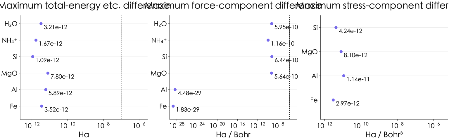
| System / paired frames | Total energy etc. / Ha | Energy components / Ha | Force / Ha·bohr⁻¹ | Stress / Ha·bohr⁻³ | Occupied levels / Ha |
|---|---|---|---|---|---|
| H₂O / 7 | Not applicable | ||||
| NH₄⁺ / 4 | Not applicable | ||||
| Si / 5 | |||||
| MgO / 5 | |||||
| Al / 5 | |||||
| Fe / 2 |
Seven H₂O frames and four NH₄⁺ frames test changing molecular geometries. Si and MgO each contribute five frames, Al five and the Fe single point two. Final summaries and intermediate geometries both enter the comparison, preserving the correspondence between forces, cell and electronic states throughout relaxation. The maximum occupied-eigenvalue difference is Ha; the maximum difference among kinetic, Hartree, exchange-correlation and pseudopotential energy components is Ha. Summed energies combine component terms whose differences can cancel; the two maxima describe agreement of aggregate quantities and individual components separately.
These differences quantify cross-runtime numerical agreement for the same method. Sampling checks and energy-derivative checks separately test the numerical quality of the basis, grids and physical quantities. Together, these three forms of evidence support the calculation. Metal eigenvalue comparisons select states with occupation above on at least one side; remaining levels are retained in the raw output for dedicated subsequent analysis.
Electronic-solver accuracy and convergence validation
Electronic-solver accuracy is evaluated from residuals, total energies and complete force arrays for fixed inputs. Comparisons include iterations near convergence and apply prespecified numerical tolerances to native and browser results.
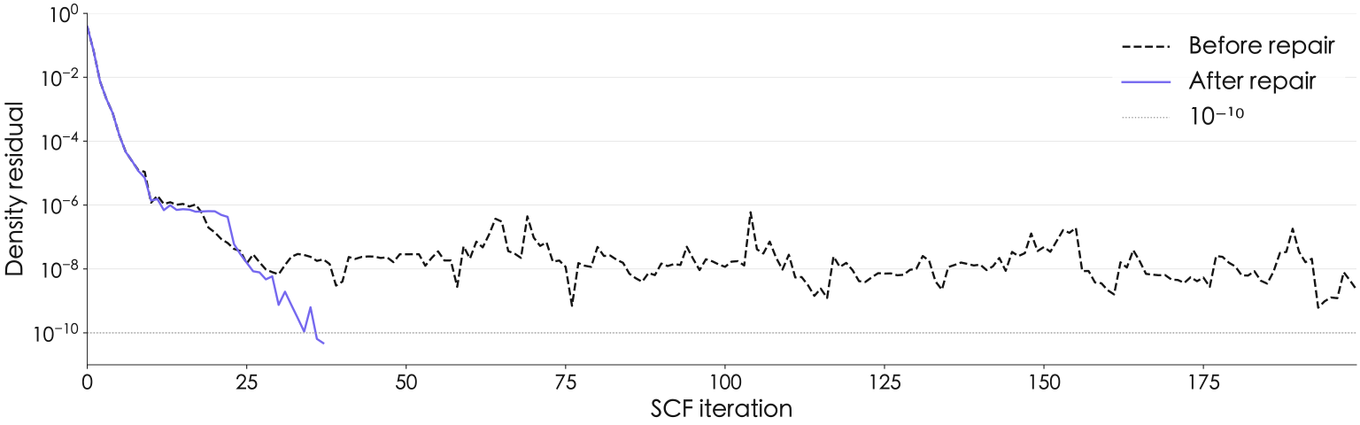
A single-variable experiment on the same MgO primitive cell fixes 20/100 Ha cutoffs, a 4×4×4 mesh, pseudopotentials, initial state and a density-residual gate. Before repair, the run reaches 200 cycles with final residuals of and . After repair, it ends in 38 cycles with and . Energy stopping, eigenvalue locking and the iteration cap retain their original settings, localizing this improvement to expansion-direction pruning.
Validation covers molecules, crystals, metals and spin-polarized systems, together with force and stress finite differences, optimization trajectories and complete field data. Resource measurements identify grid sizes, linear memory and execution times.
Self-consistency, metallic occupations and spin
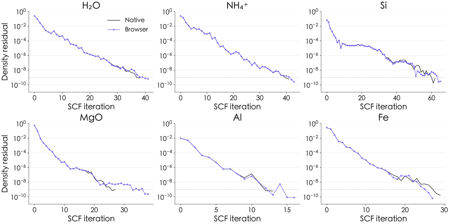
Figure 3 shows the first electronic SCF block for all six system classes. Every point comes from an actual iteration event. Native and browser runs both solve from the initial density, retaining their own iteration counts and non-monotonic behavior. Atomic relaxation of H₂O, NH₄⁺ and both crystals additionally requires the same residual checks at every geometry.
Al and Fe use Fermi occupations with width 0.01 Ha and 20×20×20 and 16×16×16 meshes, respectively. Metal relaxation uses the Helmholtz free energy as its variational quantity:
Output retains internal energy, electronic entropy and free energy separately. Occupation weights reconstruct electron count; the highest-band occupation and weighted electron tail enter the checks. The broadening specifies electronic occupations, while structural inputs specify the cell conditions.
bcc Fe starts with a spin electron imbalance of +3 and allows collinear spin to relax during the solve. Its converged is 2.2598006043, corresponding to a spin moment of approximately 2.2598 μB per one-atom primitive cell. The native/browser difference is electrons. This value is defined by the recorded PBE/GBRV configuration, initial spin and cell; electron count is independently reconstructed from occupations.
From electronic self-consistency to atomic relaxation
Atomic relaxation uses forces to update geometry, jointly testing electronic states, atom indexing and coordinate transfer. All four chains start from their actual initial geometries and retain the converged electronic state and corresponding atomic forces at each step. Native and browser trajectories are compared frame by frame; every final maximum atomic force meets the fixed Ha bohr⁻¹ threshold.
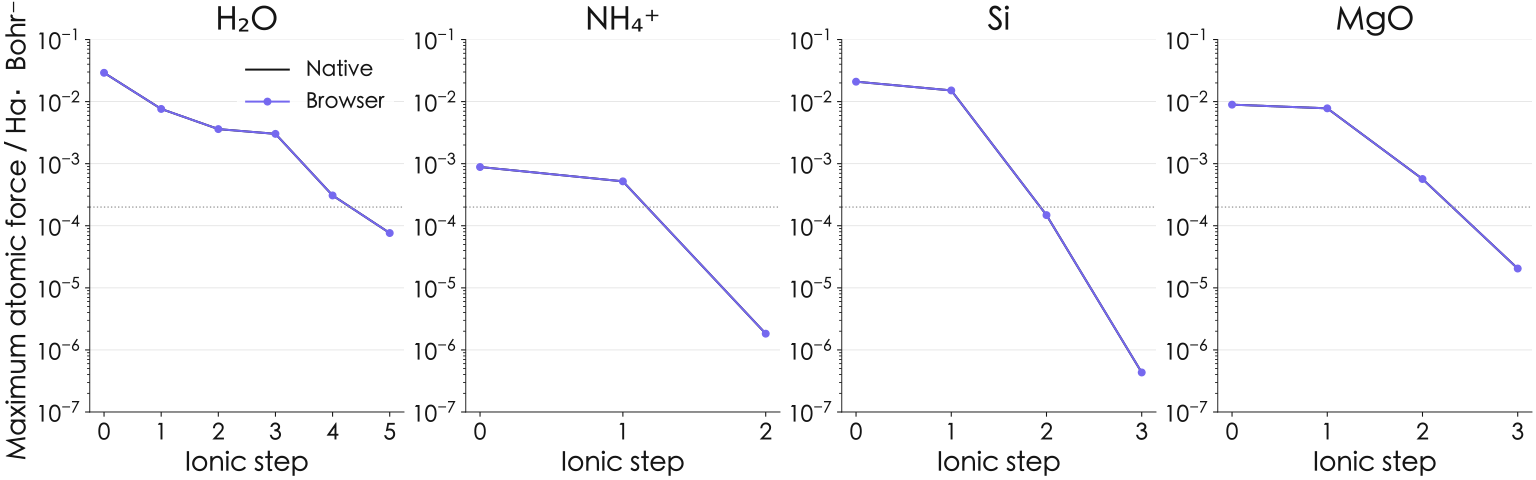
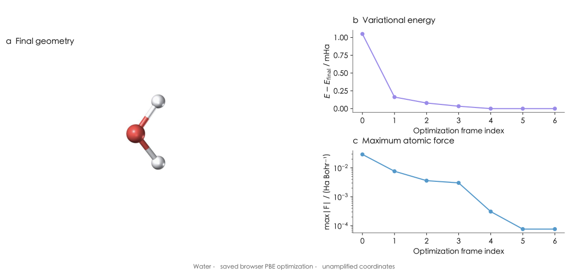
Final maximum forces are Ha bohr⁻¹ for H₂O, for NH₄⁺, for Si and for MgO. The relaxations produce 6, 3, 4 and 4 geometry-step records, respectively, plus their final summary frames. Isolated molecular cells and fixed periodic cells retain their respective physical meaning within the same record structure.
Independent energy-derivative checks of forces and stress
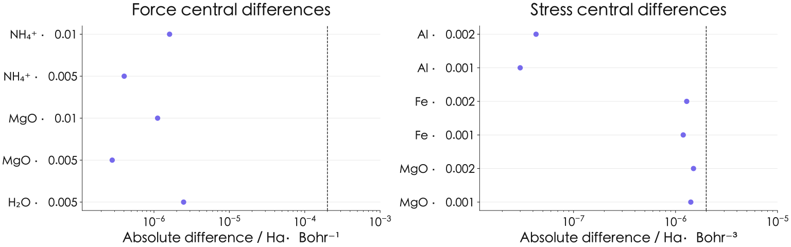
Atomic forces are checked by central differences, and stress by prescribed strain paths at fixed fractional coordinates. For lattice matrix ,
Here , stress follows the positive energy–strain derivative convention, and V is the reference volume. The Al and MgO 00 checks use Q₀₀=1 with all other components zero; isotropic Fe uses Q=I and therefore probes the stress trace. Molecules and insulators use , while metals use .
| System and derivative | Step | Analytical | Central difference | Absolute difference |
|---|---|---|---|---|
| NH₄⁺ · force / Ha·bohr⁻¹ | 0.01 | |||
| NH₄⁺ · force / Ha·bohr⁻¹ | 0.005 | |||
| MgO · force / Ha·bohr⁻¹ | 0.01 | |||
| MgO · force / Ha·bohr⁻¹ | 0.005 | |||
| Al · stress / Ha·bohr⁻³ | 0.002 | |||
| Al · stress / Ha·bohr⁻³ | 0.001 | |||
| Fe · stress / Ha·bohr⁻³ | 0.002 | |||
| Fe · stress / Ha·bohr⁻³ | 0.001 | |||
| H₂O · force / Ha·bohr⁻¹ | 0.005 | |||
| MgO · stress / Ha·bohr⁻³ | 0.002 | |||
| MgO · stress / Ha·bohr⁻³ | 0.001 |
NH₄⁺ and MgO each use atomic displacements of 0.01 and 0.005 bohr. Halving the step reduces the NH₄⁺ error from to Ha bohr⁻¹ and the MgO error from to . Both decrease by approximately fourfold, consistent with second-order central-difference truncation. The 0.005 bohr H₂O check has error Ha bohr⁻¹.
Stress checks use strain amplitudes of 0.002 and 0.001. Al 00-component errors are and Ha bohr⁻³; MgO 00-component errors are and ; isotropic Fe errors are and . All pass the predetermined Ha bohr⁻³ threshold. Complete derivative data retain both steps, analytical derivatives, positive/negative perturbation energies and the actual computational configurations.
Independent single-point verification after Al cell relaxation
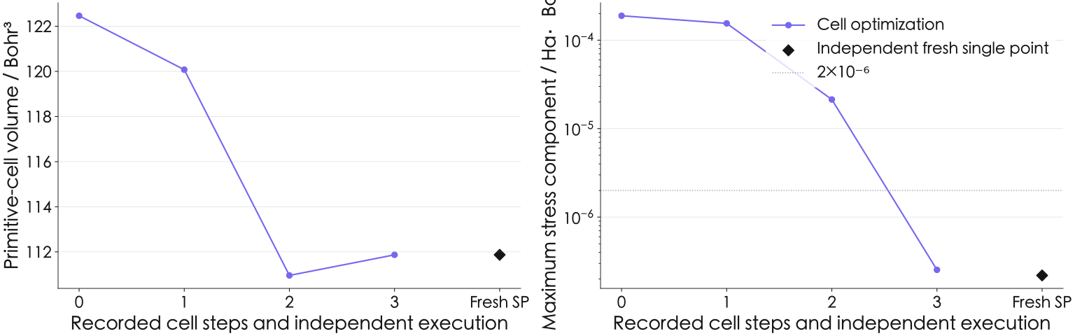
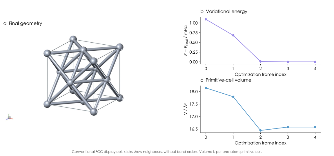
fcc Al extends the validation chain to cell degrees of freedom. The workspace calculation records a primitive-cell volume changing from 122.4653854 to 111.8697285 bohr³, corresponding to a conventional cubic lattice parameter of 4.047547845 Å. After relaxation, the workflow extracts the actual cell and coordinates from the final frame and creates a new single-point task with a new Worker. Optimizer and check records separately retain inputs, methods, result references and execution identities.
| Quantity | Browser calculation result | Native/browser absolute difference |
|---|---|---|
| Free energy / Ha | -2.1033764923615754 | |
| Maximum stress component / Ha·bohr⁻³ | ||
| Occupied levels / Ha | Complete weighted electronic-state arrays | |
| Primitive-cell volume / bohr³ | 111.8697284950 | Matches the relaxation endpoint cell |
The independent browser single point gives free energy −2.1033764923615754 Ha and maximum stress component Ha bohr⁻³. Recalculating this browser single-point input verbatim with the native program gives a free-energy difference of Ha, stress-component difference of Ha bohr⁻³ and occupied-eigenvalue difference of Ha. The check also passes electron count, occupation-tail, force and the original cell-relaxation stress criterion.
The optimizer endpoint has free energy −2.1033769126596926 Ha, differing from the fresh single point by Ha. The relaxation path and independent single point each retain their actual FFT-grid and basis settings; this difference is reported separately from native/browser porting error. The independent check establishes that a new electronic solve at the final cell still meets the original force and stress conditions.
Calculations and reusable results in the workspace
The Mol2Mat workspace provides three entry points: DFT single points, atomic relaxation and cell relaxation. Molecular coordinates and periodic cells enter through structure inputs. Electronic SCF progress is visible during execution; three-dimensional structures, relaxation trajectories and numerical results remain available afterwards. Intermediate or final frames can be used for a new single-point calculation. Derived records preserve the parent task, frame index and method, linking a relaxed structure to its subsequent electronic solve.
Workspace checks include H₂O atomic relaxation, NH₄⁺/Si/MgO single points and the Al “cell relaxation → independent single point” calculation. After saving, reopening, export, navigation and reload, content hashes preserve the association between structures, methods and execution records. Numerical validation of the Fe spin single point uses retained native/browser calculation records. A separate intentionally cancelled workspace run checks task termination, record recovery and export.
Computation runs in a dedicated Worker using single-threaded binary64 CPU WebAssembly, native WASM exceptions and a 4 GiB linear-memory ceiling. Output growth is capped at 24 MiB and the actual per-task time budget is 3600 s. Measured state, band and grid sizes are checked before successful output. Execution evidence was recorded in pinned Chrome 154.0.8037.98 on macOS. Cancellation terminates the corresponding Worker and releases resources; runtime data and saved objects retain the identity of that execution.
| Object | Calculations and numerical validation | Result storage and recovery |
|---|---|---|
| H₂O | Atomic relaxation and framewise native comparison | Save, open, return, reload; derive middle and final frames |
| NH₄⁺ / Si / MgO | Single points and complete-output validation | Save, open, return, reload; geometry and provenance retained |
| Al | Cell relaxation, fresh single point and native verification | Two saved tasks; export and recover the complete workflow |
| Fe | Retained native/browser spin single-point numerical records | Save, open, return, reload and export the intentionally cancelled run record |
Calculation versions and verification conditions
Each comparison fixes software versions, structures, pseudopotentials, cutoffs, sampling and convergence conditions, with checksums identifying calculation artifacts and outputs. Native and browser results are compared using the same observable definitions and prespecified tolerances.
The public summary CSV, derivative CSV and verification summary support checks of the numerical conclusions. Calculations can be repeated with the stated inputs and method settings, and figures can be redrawn from the corresponding numerical data.
| Component | Versions, hashes and build records |
|---|---|
| JDFTx | e305ab5de00f4b8193a503b62f314c86c36baafc |
| Emscripten / Node | 5.0.3 / 24.19.0 |
| GSL / FFTW | 2.8 / 3.3.11 |
| OpenBLAS | Native 0.3.34; fixed WASM 0.3.31 side module |
| Core source builds | 136 actual compile/link steps each for native and WASM |
| Source-file comparison | 541 source files matched individually on each side |
| JDFTx WASM | 4d1d9c735f173d1cf0492ba1c9a593ca2bc32af123ddc3d560608ae3e1a34c90 |
| Corresponding-source archive SHA-256 | 631c2c559ab1c6a4f0ce870942201afce24adfc894c769cd4d94b6fea409a9b8 |
Conclusions
Native/browser comparisons for six fixed inputs establish agreement in energies, forces, stress and electronic-state arrays under the tested conditions. Four atomic relaxations meet the prescribed force threshold. An independent browser single point and native recalculation after Al cell relaxation meet the original force and stress criteria. A matched-input comparison evaluates the Davidson cutoff revision, while independent energy differences check forces and stress.
These conclusions apply to the listed systems, PBE pseudopotential settings, sampling and convergence conditions. Numerical comparisons, sampling refinement and optimized endpoints use their respective metrics; public data support checks of summaries, derivative tables and figures.
Data and reproducibility
Energy, force and stress differences can be replotted from summary.csv. Perturbed energies and analytical derivatives in derivatives.csv support independent finite-difference checks. evidence.json provides the verification summary and result identities.
Calculation reproduction uses the recorded structures, pseudopotentials, cutoffs, sampling and stopping conditions, with results compared against observable-specific tolerances. Performance reproduction also fixes the device, parallel configuration, initialization boundary and repetition count.
Data and sources
- Complete-trajectory differences · CSV
- Energy derivatives · CSV
- Verification summary and file identities · JSON
- R. Sundararaman et al. JDFTx: Software for joint density-functional theory. SoftwareX 6, 278–284 (2017). doi:10.1016/j.softx.2017.10.006
- M. Schlipf, F. Gygi. Optimization algorithm for the generation of ONCV pseudopotentials. Computer Physics Communications 196, 36–44 (2015). doi:10.1016/j.cpc.2015.05.011
- K. F. Garrity et al. Pseudopotentials for high-throughput DFT calculations. Computational Materials Science 81, 446–452 (2014). doi:10.1016/j.commatsci.2013.08.053
- JDFTx source commit e305ab5de00f4b8193a503b62f314c86c36baafc.
- Mol2Mat retained raw numerical evidence and file identities.
- Mol2Mat: saved-data Mol* figure sources, render settings and checksums.